Customer Segmentation K Means Cluster
Customer segmentation is the process of separation of customers into groups based on common characteristics or patterns so companies can market their products to each group effectively and significantly.
In business-to-consumer marketing, most of the companies often segment their customers into Age, Gender, Marital status, location (urban, suburban, rural), Life stage (single, married, divorced, empty-nester, retired,..), etc.
Segmentation allows marketers to get better ideas about the product and Identify ways to improve existing products or new product or service opportunities, establish better customer relationships, focus on the most profitable customers, etc…
In this tutorial we are going to discuss about k means customer segmentation analysis in R.
Load Library
library(ggplot2)
library(factoextra)
library(dplyr)
Getting Data
data<-read.csv("D:/RStudio/CustomerSegmentation/Cust_Segmentation.csv",1)
str(data)
You can access the data set from here
'data.frame':       850 obs. of  10 variables:
 $ Customer.Id    : int  1 2 3 4 5 6 7 8 9 10 ...
 $ Age            : int  41 47 33 29 47 40 38 42 26 47 ...
 $ Edu            : int  2 1 2 2 1 1 2 3 1 3 ...
 $ Years.Employed : int  6 26 10 4 31 23 4 0 5 23 ...
 $ Income         : int  19 100 57 19 253 81 56 64 18 115 ...
 $ Card.Debt      : num  0.124 4.582 6.111 0.681 9.308 ...
 $ Other.Debt     : num  1.073 8.218 5.802 0.516 8.908 ...
 $ Defaulted      : int  0 0 1 0 0 NA 0 0 NA 0 ...
 $ Address        : chr  "NBA001" "NBA021" "NBA013" "NBA009" ...
 $ DebtIncomeRatio: num  6.3 12.8 20.9 6.3 7.2 10.9 1.6 6.6 15.5 4 ..
In this dataset contains total 850 observations and 10 variables.
For further analysis we need only numerical variables. Let’s make use select command from dplyr package.
data<-select(data,-Defaulted,-Address,-Customer.Id)
head(data)
Age Edu Years.Employed Income Card.Debt Other.Debt DebtIncomeRatio
1  41   2              6     19     0.124      1.073             6.3
2  47   1             26    100     4.582      8.218            12.8
3  33   2             10     57     6.111      5.802            20.9
4  29   2              4     19     0.681      0.516             6.3
5  47   1             31    253     9.308      8.908             7.2
6  40   1             23     81     0.998      7.831            10.9
Now you can see that different variables have different magnitudes, just scale the data set for further analysis.
df <- scale(data)
            Age        Edu Years.Employed     Income  Card.Debt Other.Debt DebtIncomeRatio
[1,]  0.7424783  0.3119388     -0.3785669 -0.7180358 -0.6834088 -0.5901417      -0.5761859
[2,]  1.4886141 -0.7658984      2.5722067  1.3835101  1.4136414  1.5120716       0.3911565
[3,] -0.2523695  0.3119388      0.2115878  0.2678746  2.1328854  0.8012322       1.5966138
As the k-means clustering algorithm starts with k randomly selected centroids, it’s always recommended to use the set.seed() function to get repeated results for every time when we generate the results.
Compute k-means
set.seed(123)
km.res <- kmeans(df, 3, nstart = 25)
nstart is the number of random starting partitions when centres is a number.
Always nstart > 1 is often recommended.
Optimal Cluster
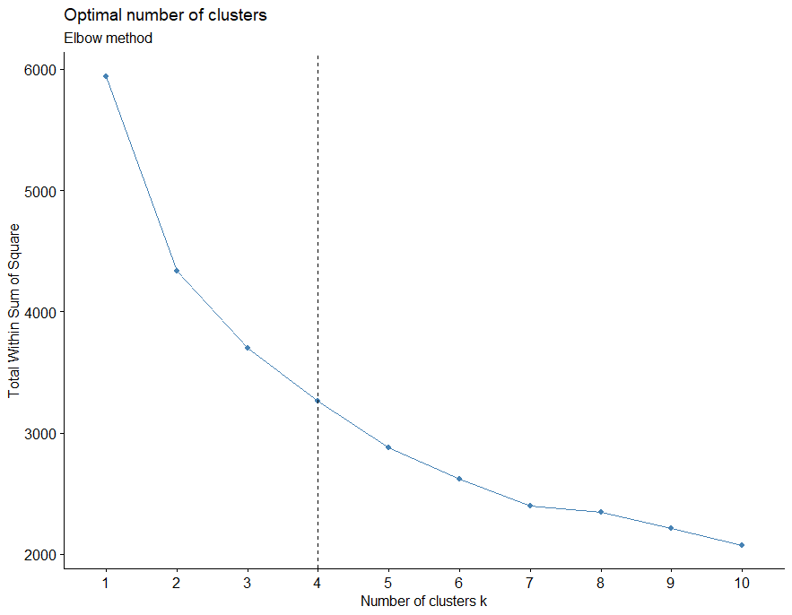
fviz_nbclust(df, kmeans, method = "wss") +
  geom_vline(xintercept = 4, linetype = 2)

Ideal cluster classification is important in customer segmentation. Let’s make use of the fviz_nbclust function in r and we can identify the optimal number of clusters.
In this case optimal number of clusters is 4.
Suppose if you want to compute the mean of each variables by clusters using the original data based on below command
aggregate(data, by=list(cluster=km.res$cluster), mean)
cluster      Age      Edu Years.Employed    Income Card.Debt Other.Debt DebtIncomeRatio
1       1 41.01316 2.223684      15.671053 113.57895 6.2833947  10.713158       18.428947
2       2 41.72664 1.598616      13.550173  59.85467 1.4986228   3.217062        8.786505
3       3 30.10103 1.696907       4.482474  28.33814 0.8858907   1.800054        9.703093
If you want to add the cluster point classifications to the original data, you can try below command
dd <- cbind(data, cluster = km.res$cluster)
head(dd)
Age Edu Years.Employed Income Card.Debt Other.Debt DebtIncomeRatio cluster
1  41   2              6     19     0.124      1.073             6.3       3
2  47   1             26    100     4.582      8.218            12.8       1
3  33   2             10     57     6.111      5.802            20.9       1
4  29   2              4     19     0.681      0.516             6.3       3
5  47   1             31    253     9.308      8.908             7.2       1
6  40   1             23     81     0.998      7.831            10.9       2
Cluster size
For identification number of cluster sizes you can make use of size command.
km.res$size
76 289 485
Cluster means
km.res$centers
Age         Edu Years.Employed     Income   Card.Debt  Other.Debt DebtIncomeRatio
1  0.7441145  0.55303394      1.0482874  1.7358161  2.21398012  2.24620091      1.22886710
2  0.8328407 -0.12068793      0.7353757  0.3419391 -0.03678407  0.04068771     -0.20613944
3 -0.6128736 -0.01474591     -0.6024606 -0.4757576 -0.32501421 -0.37622684     -0.06973114
Cluster Plot
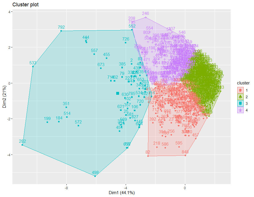
To create a beautiful graph of the clusters generated with the kmeans() function and based on ggplot2 and factoextra package.
fviz_cluster(km.res ,data = df)

Conclusion
If variables are huge, then K-Means most of the times computationally faster than hierarchical clustering, if we keep k smalls, use customer segmentation based on k means and maximize business profits.


