Gradient Boosting in R

Gradient Boosting in R, in this tutorial we are going to discuss extreme gradient boosting.

Why is eXtreme Gradient Boosting in R?

Popular in machine learning challenges.

Fast and accurate

Can handle missing values.

Is it requires numeric inputs?

Yes, eXtreme Gradient Boosting requires a numeric matrix for its input.

Sample Size calculation formula

Load Library

library(xgboost)
library(magrittr)
library(dplyr)
library(Matrix)

Getting Data

data <- read.csv("D:/RStudio/NaiveClassifiaction/binary.csv", header = T)
str(data)

'data.frame': 400 obs. of  4 variables:
 $ admit: int  0 1 1 1 0 1 1 0 1 0 ...
 $ gre  : int  380 660 800 640 520 760 560 400 540 700 ...
 $ gpa  : num  3.61 3.67 4 3.19 2.93 3 2.98 3.08 3.39 3.92 ...
 $ rank : int  3 3 1 4 4 2 1 2 3 2 ...

Data set contains total 400 obsevations and 4 variables. eXtreme Boosting requires numerical variable, so just convert rank data into factor variables.

Measures of Central Tendency

data$rank <- as.factor(data$rank)

Partition data

Let’s partition the data sets into train data and test data.

set.seed(1234)
ind <- sample(2, nrow(data), replace = T, prob = c(0.8, 0.2))
train <- data[ind==1,]
test <- data[ind==2,]

 Matrix Creation

In this case Rank variable is factor variable required hot encoding for the same. Based on hot encoding factor variables convert into dummy variable.

What is business forecasting?

trainm <- sparse.model.matrix(admit ~ .-1, data = train)
head(trainm)

6 x 6 sparse Matrix of class "dgCMatrix"
  gre  gpa rank1 rank2 rank3 rank4
1 380 3.61     .     .     1     .
2 660 3.67     .     .     1     .
3 800 4.00     1     .     .     .
4 640 3.19     .     .     .     1
6 760 3.00     .     1     .     .
7 560 2.98     1     .     .     .

train_label <- train[,"admit"]
train_matrix <- xgb.DMatrix(data = as.matrix(trainm), label = train_label)

Now we converted train data sets in to necessary format., sameway we need to convert into test data also.

testm <- sparse.model.matrix(admit~.-1, data = test)
test_label <- test[,"admit"]
test_matrix <- xgb.DMatrix(data = as.matrix(testm), label = test_label)

Parameters

nc <- length(unique(train_label))

Basically 2 different classes in the train label datset

xgb_params <- list("objective" = "multi:softprob",
                   "eval_metric" = "mlogloss",
                   "num_class" = nc)
watchlist <- list(train = train_matrix, test = test_matrix)

watch list will help us to identify the error in each iteration.

Naive Bayes Classification in R

Gradient Boosting in R

bst_model <- xgb.train(params = xgb_params,
                       data = train_matrix,
                       nrounds = 1000,
                       watchlist = watchlist,
                       eta = 0.001,
                       max.depth = 3,
                       gamma = 0,
                       subsample = 1,
                       colsample_bytree = 1,
                       missing = NA,
                       seed = 333)

##### xgb.Booster
raw: 2.4 Mb
call:
  xgb.train(params = xgb_params, data = train_matrix, nrounds = 1000,
    watchlist = watchlist, eta = 0.001, max.depth = 3, gamma = 0,
    subsample = 1, colsample_bytree = 1, missing = NA, seed = 333)
params (as set within xgb.train):
  objective = "multi:softprob", eval_metric = "mlogloss", num_class = "2", eta = "0.001", 
ax_depth = "3", gamma = "0", subsample = "1", colsample_bytree = "1", missing = "NA", seed = 
333", validate_parameters = "TRUE"
xgb.attributes:
  niter
callbacks:
  cb.print.evaluation(period = print_every_n)
  cb.evaluation.log()
# of features: 6
niter: 1000
nfeatures : 6
evaluation_log:
    iter train_mlogloss test_mlogloss
       1       0.692889      0.692974
       2       0.692631      0.692793
---                                 
     999       0.556583      0.625728
    1000       0.556514      0.625710

Training & test error plot

e <- data.frame(bst_model$evaluation_log)
plot(e$iter, e$train_mlogloss, col = 'blue')
lines(e$iter, e$test_mlogloss, col = 'red')

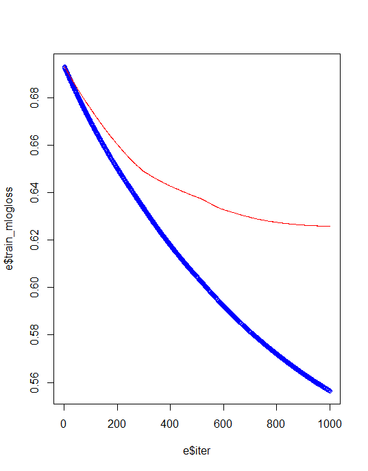
For avoiding overfiiting and best model creation we need to identify best iteration and eta values.

min(e$test_mlogloss)
e[e$test_mlogloss == 0. 613294,]

We can rerun the model based on above values.

LSTM Networks in R

Gradient Boosting in R

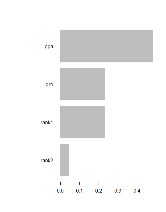
bst_model <- xgb.train(params = xgb_params,
                       data = train_matrix,
                       nrounds = 2,
                       watchlist = watchlist,
                       eta = 0.613294,
                       max.depth = 3,
                       gamma = 0,
                       subsample = 1,
                       colsample_bytree = 1,
                       missing = NA,
                       seed = 333)
Feature importance
imp <- xgb.importance(colnames(train_matrix), model = bst_model)
print(imp)

Feature       Gain      Cover  Frequency
1:     gpa 0.48632797 0.47722628 0.35714286
2:     gre 0.23495920 0.32849509 0.42857143
3:   rank1 0.23432569 0.17282919 0.14285714
4:   rank2 0.04438714 0.02144944 0.07142857

xgb.plot.importance(imp)

Prediction & confusion matrix

p <- predict(bst_model, newdata = test_matrix)

Pred <- matrix(p, nrow = nc, ncol = length(p)/nc) %>%
         t() %>%
         data.frame() %>%
         mutate(label = test_label, max_prob = max.col(., "last")-1)

          X1        X2 label max_prob
1  0.7780407 0.2219593     0        0
2  0.6580867 0.3419133     0        0
3  0.6111851 0.3888150     0        0
4  0.4440117 0.5559883     1        1
5  0.6111851 0.3888150     1        0
6  0.4345139 0.5654861     1        1
7  0.7780407 0.2219593     1        0
8  0.7780407 0.2219593     1        0
9  0.6580867 0.3419133     0        0
10 0.6580867 0.3419133     1        0
11 0.6159363 0.3840637     0        0
12 0.6580867 0.3419133     0        0
13 0.7780407 0.2219593     0        0
14 0.5099485 0.4900515     1        0
15 0.4440117 0.5559883     1        1
16 0.7780407 0.2219593     0        0
17 0.5099485 0.4900515     0        0
18 0.6111851 0.3888150     1        0
19 0.7780407 0.2219593     1        0
20 0.7780407 0.2219593     0        0
21 0.7780407 0.2219593     0        0
22 0.6580867 0.3419133     1        0
23 0.7780407 0.2219593     0        0
24 0.8379621 0.1620379     0        0
25 0.1789861 0.8210139     1        1
26 0.6111851 0.3888150     1        0
27 0.7780407 0.2219593     1        0
28 0.6111851 0.3888150     0        0
29 0.6580867 0.3419133     1        0
30 0.1789861 0.8210139     1        1
31 0.5099485 0.4900515     0        0
32 0.7780407 0.2219593     0        0
33 0.6111851 0.3888150     0        0
34 0.6111851 0.3888150     0        0
35 0.7581326 0.2418674     0        0
36 0.6111851 0.3888150     1        0
37 0.6111851 0.3888150     0        0
38 0.6580867 0.3419133     0        0
39 0.6111851 0.3888150     0        0
40 0.6111851 0.3888150     0        0
41 0.6580867 0.3419133     1        0
42 0.6111851 0.3888150     1        0
43 0.6111851 0.3888150     0        0
44 0.7780407 0.2219593     0        0
45 0.6111851 0.3888150     0        0
46 0.7780407 0.2219593     0        0
47 0.6111851 0.3888150     0        0
48 0.6580867 0.3419133     0        0
49 0.6111851 0.3888150     0        0
50 0.6111851 0.3888150     0        0
51 0.7780407 0.2219593     0        0
52 0.6111851 0.3888150     0        0
53 0.6111851 0.3888150     1        0
54 0.6159363 0.3840637     0        0
55 0.6111851 0.3888150     0        0
........................
75 0.5099485 0.4900515     0        0

0 indicates student not admitted and 1 indicates students admitted in the program.

table(Prediction = pred$max_prob, Actual = pred$label)

        Actual
Prediction  0  1
         0 49 20
         1  1  5

Conclusion

Based on this tutorial you can make use of eXtreme Gradient Boosting machine algorithm applications very easily, in this case model accuracy is around 72%.

Market Basket Analysis in R