Timeseries analysis in R
Timeseries analysis in R, in statistics time series, is one of the vast subjects, here we are going to analyze some basic functionalities with the help of R software.
The idea here is to how to start time series analysis in R. In this tutorial will go through different areas like decomposition, forecasting, clustering, and classification.
Getting Time series data
data("AirPassengers")
AP <- AirPassengers
str(AP)
Time-Series [1:144] from 1949 to 1961: 112 118 132 129 121 135 148 148 136 119 ...
Year is starting from 1949 and ending with 1961 with 144 observations.
Now we need to convert the dataset into timeseries data.
ts(AP, frequency = 12, start=c(1949,1))
Jan Feb Mar Apr May Jun Jul Aug Sep Oct Nov Dec
1949 112 118 132 129 121 135 148 148 136 119 104 118
1950 115 126 141 135 125 149 170 170 158 133 114 140
1951 145 150 178 163 172 178 199 199 184 162 146 166
1952 171 180 193 181 183 218 230 242 209 191 172 194
1953 196 196 236 235 229 243 264 272 237 211 180 201
1954 204 188 235 227 234 264 302 293 259 229 203 229
1955 242 233 267 269 270 315 364 347 312 274 237 278
1956 284 277 317 313 318 374 413 405 355 306 271 306
1957 315 301 356 348 355 422 465 467 404 347 305 336
1958 340 318 362 348 363 435 491 505 404 359 310 337
1959 360 342 406 396 420 472 548 559 463 407 362 405
1960 417 391 419 461 472 535 622 606 508 461 390 432
plot(AP)

This data looks stationary and we can go for log transformation for nonstationary data.
Timeseries analysis in R
Log transform
AP <- log(AP)
plot(AP)

Decomposition of additive time series
Major components of time series
decomp <- decompose(AP)
decomp$figure
[1] -0.085815019 -0.114412848 0.018113355 -0.013045611 -0.008966106 0.115392997 0.210816435 0.204512399 0.064836351 -0.075271265 -0.215845612 -0.100315075
plot(decomp$figure,
     type = 'b',
     xlab = 'Month',
     ylab = 'Seasonality Index',
     col = 'blue',
     las = 2)
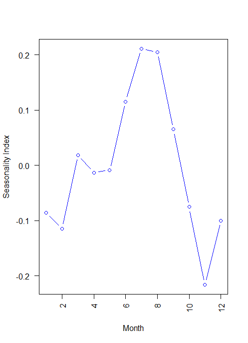
In this dataset currently in log form, Month 11 showing -20% downside, and Month 7 and 8 showing 20% upper side.
plot(decomp)

Basically, the time series split into three component trend, seasonal and random.
Forecasting
ARIMA – Autoregressive Integrated Moving Average
library(forecast)
model <- auto.arima(AP)
model
Series: AP
ARIMA(0,1,1)(0,1,1)[12]
Coefficients:
          ma1     sma1
      -0.4018  -0.5569
s.e.   0.0896   0.0731
sigma^2 estimated as 0.001371:  log likelihood=244.7
AIC=-483.4   AICc=-483.21   BIC=-474.77
AIC and BIC will help us to choose the best time series model.
Repeated Measures of ANOVA in R
ACF and PACF plots
It is always looking into ACF and PACF when we are dealing with time series data.
acf(model$residuals, main = 'Correlogram')

The dotted lines are significant bounds. A log 0 its crossing the significance bound.
Within 1 and 1.5 its just touching the significance bounds
pacf(model$residuals, main = 'Partial Correlogram' )

In this case all the lags are within significant bounds.
Ljung-Box test
Box.test(model$residuals, lag=20, type = 'Ljung-Box')
Box-Ljung test
data:  model$residuals
X-squared = 17.688, df = 20, p-value = 0.6079
No significant difference was observed that indicates autocorrelation observed at lag 1 and 1.5 may be due to random chance.
Residual plot
hist(model$residuals,
     col = 'red',
     xlab = 'Error',
     main = 'Histogram of Residuals',
     freq = FALSE)
lines(density(model$residuals))

Most of the values are concentrated at 0 and look normal distribution, same indicates there is no series problem with the existing model.
Forecast
f <- forecast(model, 48)
library(ggplot2)
autoplot(f)

accuracy(f)
                  ME       RMSE        MAE        MPE      MAPE      MASE       ACF1
Training set 0.0005730622 0.03504883 0.02626034 0.01098898 0.4752815 0.2169522 0.01443892
Time-series clustering
Getting Data for Cluster Analysis
The dataset you can access from here
data <- read.table("D:/RStudio/TimeseriesAnalysis/synthetic_control.data.txt", header = F, sep = "")
str(data)
'data.frame': 600 obs. of  60 variables:
plot(data[,60], type = 'l')

j <- c(5, 105, 205, 305, 405, 505)
sample <- t(data[j,]) plot.ts(sample,
main = "Time-series Plot",
col = 'blue',
type = 'b')

Data preparation
n <- 10
s <- sample(1:100, n)
i <- c(s,100+s, 200+s, 300+s, 400+s, 500+s)
d <- data[i,]
str(d)
pattern <- c(rep('Normal', n),
             rep('Cyclic', n),
             rep('Increasing trend', n),
             rep('Decreasing trend', n),
             rep('Upward shift', n),
             rep('Downward shift', n))
Calculate distances
library(dtw)
distance <- dist(d, method = "DTW")
Hierarchical clustering
hc <- hclust(distance, method = 'average')
plot(hc,
     labels = pattern,
     cex = 0.7,
     hang = -1,
     col = 'blue')
rect.hclust(hc, k=4)

Time series classification
Data preparation
pattern100 <- c(rep('Normal', 100),
                rep('Cyclic', 100),
                rep('Increasing trend', 100),
                rep('Decreasing trend', 100),
                rep('Upward shift', 100),
                rep('Downward shift', 100))
newdata <- data.frame(data, pattern100)
str(newdata)
newdata$pattern100<-factor(newdata$pattern100)
Classification with decision tree
library(party)
tree <- ctree(pattern100~., newdata)
Classification performance
tab <- table(Predicted = predict(tree, newdata), Actual = newdata$pattern100)
Actual
Predicted          Cyclic Decreasing trend Downward shift Increasing trend Normal
  Cyclic               97                0              3                0      0
  Decreasing trend      0               99              8                0      0
  Downward shift        0                1             89                0      0
  Increasing trend      2                0              0               96      0
  Normal                1                0              0                0    100
  Upward shift          0                0              0                4      0
                  Actual
Predicted          Upward shift
  Cyclic                      0
  Decreasing trend            0
  Downward shift              0
  Increasing trend            6
  Normal                      4
  Upward shift               90
sum(diag(tab))/sum(tab)
0.9516667
This indicates classification is above 95% accurate.


Is anyone here in a position to recommend Realistic Dildos? Thanks x