Deep Neural Network in R
Deep Neural Network in R, Neural Network is just like a human nervous system, which is made up of interconnected neurons, in other words, a neural network is made up of interconnected information processing units.
The neural network draws from the parallel processing of information, which is the strength of this method.
A neural network helps us to extract meaningful information and detect hidden patterns from complex data sets.
A neural network is considered one of the most powerful techniques in the data science world.
This method is developed to solve problems that are easy for humans and difficult for machines. For example, identifying pictures like dogs and cats. These problems are often referred to as pattern recognition.
Let’s see the Implementation of a Neural Network in R
Naïve Bayes Classification In r
Load Library
library(keras)
library(mlbench)
library(dplyr)
library(magrittr)
library(neuralnet)
Getting Data
data("BostonHousing")
data <- BostonHousing
str(data)
'data.frame': 506 obs. of 14 variables: $ crim : num 0.00632 0.02731 0.02729 0.03237 0.06905 ... $ zn : num 18 0 0 0 0 0 12.5 12.5 12.5 12.5 ... $ indus : num 2.31 7.07 7.07 2.18 2.18 2.18 7.87 7.87 7.87 7.87 ... $ chas : Factor w/ 2 levels "0","1": 1 1 1 1 1 1 1 1 1 1 ... $ nox : num 0.538 0.469 0.469 0.458 0.458 0.458 0.524 0.524 0.524 0.524 ... $ rm : num 6.58 6.42 7.18 7 7.15 ... $ age : num 65.2 78.9 61.1 45.8 54.2 58.7 66.6 96.1 100 85.9 ... $ dis : num 4.09 4.97 4.97 6.06 6.06 ... $ rad : num 1 2 2 3 3 3 5 5 5 5 ... $ tax : num 296 242 242 222 222 222 311 311 311 311 ... $ ptratio: num 15.3 17.8 17.8 18.7 18.7 18.7 15.2 15.2 15.2 15.2 ... $ b : num 397 397 393 395 397 ... $ lstat : num 4.98 9.14 4.03 2.94 5.33 ... $ medv : num 24 21.6 34.7 33.4 36.2 28.7 22.9 27.1 16.5 18.9 ...
In this data set contains 506 observations and 14 variables. The variables chas as a factor variable, we need to convert in into numerical variable because neural network handles only numerical data.
Let us understand the data set, Medv is the response variable, and the remaining are the predictors.
We need to convert factor variables into numeric variables while using the below-mentioned command. This function automatically detects the factor variables and convert them into numerical variables.
data %<>% mutate_if(is.factor, as.numeric)
Neural Network in R Visualization
In the model creation we need to mention the hidden layers, in this cae we use 12 nuerons in the first layer and 7 nurons in the second layer
n <- neuralnet(medv ~ crim+zn+indus+chas+nox+rm+age+dis+rad+tax+ptratio+b+lstat,
               data = data,
               hidden = c(12,7),
               linear.output = F,
               lifesign = 'full',
               rep=1)
Plot the model visual identification
plot(n,col.hidden = 'darkgreen',
col.hidden.synapse = 'darkgreen',
     show.weights = F,
     information = F,
     fill = 'lightblue')
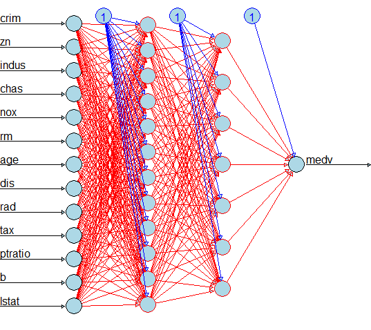
Now we can see each predictor variable has one neuron, the first layer has 12 neurons, the second layer has 7 neurons and the out variable has one neuron.
Just convert the data frame into matrix for further analysis.
data <- as.matrix(data)
dimnames(data) <- NULL
Data Partition
The data set need to partition test test data and training data set.
set.seed(123)
ind <- sample(2, nrow(data), replace = T, prob = c(.7, .3))
training <- data[ind==1,1:13]
test <- data[ind==2, 1:13]
trainingtarget <- data[ind==1, 14]
testtarget <- data[ind==2, 14]
str(trainingtarget)
num [1:363] 24 34.7 28.7 22.9 16.5 18.9 18.9 21.7 20.4 18.2 ...
str(testtarget)
num [1:143] 21.6 33.4 36.2 27.1 15 19.9 18.2 13.6 14.5 13.9 ...
Scaling
The neural network requires normalized values for better prediction, just normalize or scale the predictor variables based on below function
m <- colMeans(training)
s <- apply(training, 2, sd)
training <- scale(training, center = m, scale = s)
test <- scale(test, center = m, scale = s)
Model Creation
model <- keras_model_sequential()
model %>%
         layer_dense(units = 5, activation = 'relu', input_shape = c(13)) %>%
         layer_dense(units = 1)
relu stands for rectified linear unit and model we are testing one hidden layer with 5 neurons, 13 predictor variables and 1 output neuron.
Repeated Measures of ANOVA in R
Model: "sequential" _______________________________________________________________________________________________ ____________________________________________ Layer (type) Output hape Param # =============================================================================================== ============================================ dense_1 (Dense) (None, ) 70 _______________________________________________________________________________________________ ____________________________________________ dense (Dense) (None, ) 6 =============================================================================================== ============================================ Total params: 76 Trainable params: 76 Non-trainable params: 0 _______________________________________________________________________________________________ ____________________________________________
Model Compilation
model %>% compile(loss = 'mse',
optimizer = 'rmsprop',
metrics = 'mae')
Model Fitting
mymodel <- model %>%
fit(training,trainingtarget,
             epochs = 100,
             batch_size = 32,
             validation_split = 0.2)
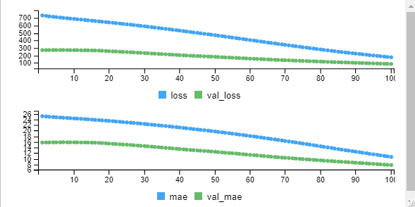
From the graph we can observe that initially the error is high and minimized at the end. The loss value you can observe from the output also over a period of time losss is decreasing.
Epoch 1/100
10/10 [==============================] - 1s 92ms/step - loss: 734.2240 - mae: 25.1547 -
al_loss: 271.0404 - val_mae: 15.7447
Epoch 2/100
10/10 [==============================] - 0s 21ms/step - loss: 727.2393 - mae: 25.0363 -
al_loss: 271.7035 - val_mae: 15.7791
Epoch 3/100
10/10 [==============================] - 0s 16ms/step - loss: 721.6415 - mae: 24.9437 -
al_loss: 272.0933 - val_mae: 15.8027
Epoch 4/100
10/10 [==============================] - 0s 35ms/step - loss: 716.5717 - mae: 24.8579 -
al_loss: 272.3845 - val_mae: 15.8226
Epoch 5/100
10/10 [==============================] - 0s 35ms/step - loss: 711.5942 - mae: 24.7728 -
al_loss: 272.1657 - val_mae: 15.8225
Epoch 6/100
10/10 [==============================] - 0s 18ms/step - loss: 706.8410 - mae: 24.6912 -
al_loss: 272.2704 - val_mae: 15.8342Epoch 7/100
10/10 [==============================] - 0s 17ms/step - loss: 701.8980 - mae: 24.6061 - val_loss: 273.0846 - val_mae: 15.8719
Epoch 8/100
10/10 [==============================] - 0s 17ms/step - loss: 696.6748 - mae: 24.5191 - val_loss: 271.7730 - val_mae: 15.8318
Epoch 9/100
10/10 [==============================] - 0s 16ms/step - loss: 692.5706 - mae: 24.4432 - val_loss: 271.6264 - val_mae: 15.8328
Epoch 10/100
10/10 [==============================] - 0s 16ms/step - loss: 688.1098 - mae: 24.3619 - val_loss: 271.1543 - val_mae: 15.8226
Epoch 11/100
10/10 [==============================] - 0s 19ms/step - loss: 683.6657 - mae: 24.2823 - val_loss: 270.8098 - val_mae: 15.8173
Epoch 12/100
.
.
.
Epoch 99/100
10/10 [==============================] - 0s 16ms/step - loss: 180.3299 - mae: 10.8129 - val_loss: 87.9922 - val_mae: 7.8188
Epoch 100/100
10/10 [==============================] - 0s 17ms/step - loss: 176.1795 - mae: 10.6425 - val_loss: 86.4092 - val_mae: 7.7314
Prediction
model %>% evaluate(test, testtarget)
pred <- model %>% predict(test)
5/5 [==============================] - 0s 1ms/step -
loss: 121.2298 - mae: 9.0212 loss
mae 121.229843   9.021233
mean((testtarget-pred)^2)
[1] 121.2298
Scatter Plot Original vs Predicted
plot(testtarget, pred)
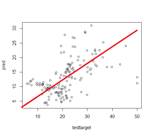
In the above, if we are drawing a straight line and all the observations are close to that line indicates the data is ideal for prediction otherwise needs improvement.
Let’s see how to increase the model prediction, make some changes in the script and rerun the model.
Under model creation you can make below changes.
model %>%
         layer_dense(units = 100, activation = 'relu', input_shape = c(13)) %>%
        layer_dropout(rate=0.4)  %>%
        layer_dense(units = 50, activation = 'relu')  %>%
        layer_dropout(rate=0.2)  %>%
         layer_dense(units = 1)
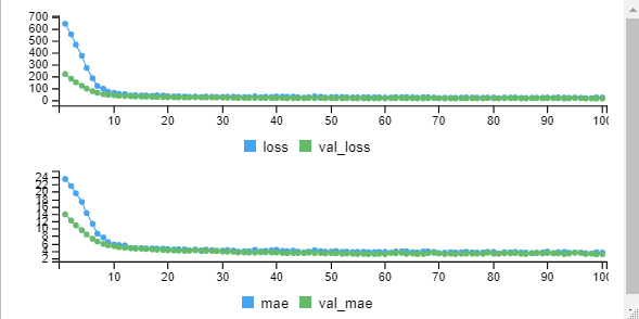
loss        mae
12.332542 2.475609
Conclusion
Based on a deep neural network, we are able to generate the model with very good loss ie. 12%. In the initial model, the error was very high around 121 and we reduced it to 12%.
Don’t forget to show your love, Subscribe the Newsletter and COMMENT below!
[newsletter_form type="minimal"]
