Cluster Analysis in R
Cluster Analysis in R, when we do data analytics, there are two kinds of approaches one is supervised and another is unsupervised.
Clustering is a method for finding subgroups of observations within a data set.
When we are doing clustering, we need observations in the same group with similar patterns and observations in different groups to be dissimilar.
If there is no response variable, then suitable for an unsupervised method, which implies that it seeks to find relationships between the n observations without being trained by a response variable.
Clustering allows us to identify homogenous groups and categorize them from the dataset.
One of the simplest clusterings is K-means, the most commonly used clustering method for splitting a dataset into a set of n groups.
If datasets contain no response variable and with many variables then it comes under an unsupervised approach.
Cluster analysis is an unsupervised approach and sed for segmenting markets into groups of similar customers or patterns.
Cluster Analysis in R
Getting Data
mydata <- read.csv("D:/RStudio/ClusterAnalysis/ClusterData.csv", header=T)
str(mydata)
'data.frame': 22 obs. of 9 variables: $ Company : chr "Arizona " "Boston " "Central " "Commonwealth" ... $ Fixed_charge: num 1.06 0.89 1.43 1.02 1.49 1.32 1.22 1.1 1.34 1.12 ... $ RoR : num 9.2 10.3 15.4 11.2 8.8 13.5 12.2 9.2 13 12.4 ... $ Cost : int 151 202 113 168 192 111 175 245 168 197 ... $ Load : num 54.4 57.9 53 56 51.2 60 67.6 57 60.4 53 ... $ D.Demand : num 1.6 2.2 3.4 0.3 1 -2.2 2.2 3.3 7.2 2.7 ... $ Sales : int 9077 5088 9212 6423 3300 11127 7642 13082 8406 6455 ... $ Nuclear : num 0 25.3 0 34.3 15.6 22.5 0 0 0 39.2 ... $ Fuel_Cost : num 0.628 1.555 1.058 0.7 2.044 ...
head(mydata)
Company Fixed_charge  RoR Cost Load D.Demand Sales Nuclear Fuel_Cost
1     Arizona          1.06  9.2  151 54.4      1.6  9077     0.0     0.628
2      Boston          0.89 10.3  202 57.9      2.2  5088    25.3     1.555
3     Central          1.43 15.4  113 53.0      3.4  9212     0.0     1.058
4 Commonwealth         1.02 11.2  168 56.0      0.3  6423    34.3     0.700
5    Con Ed NY         1.49  8.8  192 51.2      1.0  3300    15.6     2.044
6     Florida          1.32 13.5  111 60.0     -2.2 11127    22.5     1.241
pairs(mydata[2:9])
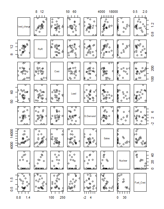
Basically, a pairs plot will provide a scatter plot for all possible combinations
Scatter plot
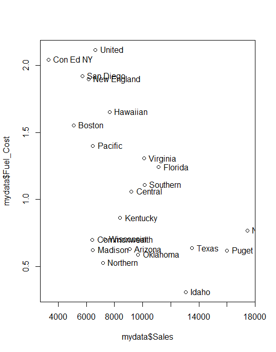
If you want to look at the scatterplot separately you can use below codes.
plot(mydata$Fuel_Cost~ mydata$Sales, data = mydata)
with(mydata,text(mydata$Fuel_Cost ~ mydata$Sales, labels=mydata$Company,pos=4))
Normalize
Normalization is very important in cluster analysis, sometimes we have variables in different scales, need to normalized based on scale function before clustering the data sets.
Naïve Bayes Classification in R
Normalization is mandatory for cluster analysis.
z <- mydata[,-c(1,1)]
means <- apply(z,2,mean)
sds <- apply(z,2,sd)
nor <- scale(z,center=means,scale=sds)
Calculate distance matrix
distance = dist(nor)
Hierarchical agglomerative clustering
mydata.hclust = hclust(distance)
plot(mydata.hclust)
plot(mydata.hclust,labels=mydata$Company,main='Default from hclust')
plot(mydata.hclust,hang=-1, labels=mydata$Company,main='Default from hclust')
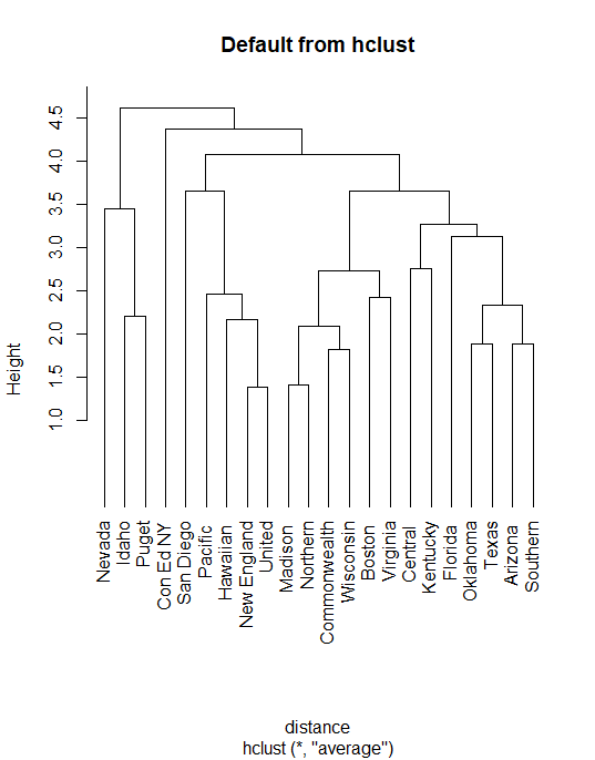
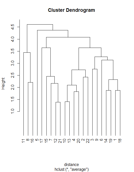
Hierarchical agglomerative clustering using “average” linkage
mydata.hclust<-hclust(distance,method="average")
plot(mydata.hclust,hang=-1)
Cluster membership
member = cutree(mydata.hclust,3)
table(member)
member
 1  2  3
18  1  3
Characterizing clusters
aggregate(nor,list(member),mean)
Group.1 Fixed_charge        RoR       Cost       Load   D.Demand      Sales    Nuclear   Fuel_Cost
1       1  -0.01313873  0.1868016 -0.2552757  0.1520422 -0.1253617 -0.2215631  0.1071944  0.06692555
2       2   2.03732429 -0.8628882  0.5782326 -1.2950193 -0.7186431 -1.5814284  0.2143888  1.69263800
3       3  -0.60027572 -0.8331800  1.3389101 -0.4805802  0.9917178  1.8565214 -0.7146294 -0.96576599
aggregate(mydata[,-c(1,1)],list(member),mean)
Group.1 Fixed_charge       RoR     Cost     Load D.Demand    Sales Nuclear Fuel_Cost
1       1     1.111667 11.155556 157.6667 57.65556 2.850000  8127.50    13.8 1.1399444
2       2     1.490000  8.800000 192.0000 51.20000 1.000000  3300.00    15.6 2.0440000
3       3     1.003333  8.866667 223.3333 54.83333 6.333333 15504.67     0.0 0.5656667
Silhouette Plot
library(cluster)
plot(silhouette(cutree(mydata.hclust,3), distance))
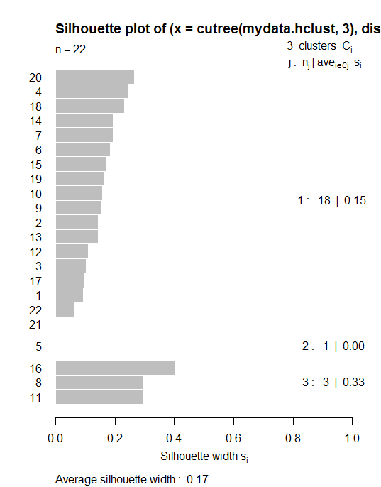
Based on the above plot, if any bar comes as negative side then we can conclude particular data is an outlier can remove from our analysis
Scree Plot
Scree plot will allow us to see the variabilities in clusters, suppose if we increase the number of clusters within-group sum of squares will come down.
wss <- (nrow(nor)-1)*sum(apply(nor,2,var))
for (i in 2:20) wss[i] <- sum(kmeans(nor, centers=i)$withinss)
plot(1:20, wss, type="b", xlab="Number of Clusters", ylab="Within groups sum of squares")
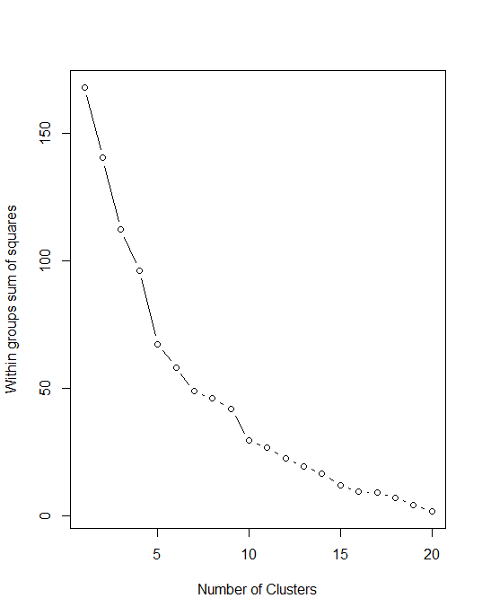
So in this data ideal number of clusters should be 3, 4, or 5.
K-means clustering
set.seed(123)
kc<-kmeans(nor,3)
kc
K-means clustering with 3 clusters of sizes 7, 5, 10
Cluster means:
  Fixed_charge         RoR       Cost       Load    D.Demand      Sales    Nuclear  Fuel_Cost
1  -0.23896065 -0.65917479  0.2556961  0.7992527 -0.05435116 -0.8604593 -0.2884040  1.2497562
2   0.51980100  1.02655333 -1.2959473 -0.5104679 -0.83409247  0.5120458 -0.4466434 -0.3174391
3  -0.09262805 -0.05185431  0.4689864 -0.3042429  0.45509205  0.3462986  0.4252045 -0.7161098
Clustering vector:
 [1] 3 1 2 3 1 2 1 3 3 3 3 1 3 2 1 3 1 2 2 3 1 3
Within cluster sum of squares by cluster:
[1] 34.16481 15.15613 57.53424
 (between_SS / total_SS =  36.4 %)
Available components:
[1] "cluster"      "centers"      "totss"        "withinss"     "tot.withinss" "betweenss"    "size"         "iter"         "ifault"
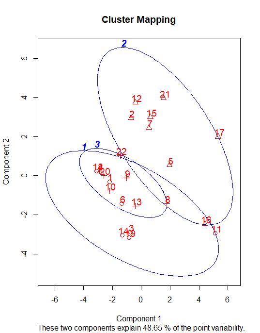
ot<-nor
datadistshortset<-dist(ot,method = "euclidean")
hc1 <- hclust(datadistshortset, method = "complete" )
pamvshortset <- pam(datadistshortset,4, diss = FALSE)
clusplot(pamvshortset, shade = FALSE,labels=2,col.clus="blue",col.p="red",span=FALSE,main="Cluster Mapping",cex=1.2)
Cluster Analysis in R
library(factoextra)
k2 <- kmeans(nor, centers = 3, nstart = 25)
We can execute k-means in R with the help of kmeans function.
The kmeans function also has a nstart option that attempts multiple initial configurations and reports on the best output.
For example, adding nstart = 25 will generate 25 initial configurations. This approach is often recommended.
str(k2)
List of 9
 $ cluster     : int [1:22] 1 2 1 1 2 1 2 3 1 1 ...
 $ centers     : num [1:3, 1:8] 0.289 -0.239 -0.6 0.593 -0.659 ...
  ..- attr(*, "dimnames")=List of 2
  .. ..$ : chr [1:3] "1" "2" "3"
  .. ..$ : chr [1:8] "Fixed_charge" "RoR" "Cost" "Load" ...
 $ totss       : num 168
 $ withinss    : num [1:3] 58.01 34.16 9.53
 $ tot.withinss: num 102
 $ betweenss   : num 66.3
 $ size        : int [1:3] 12 7 3
 $ iter        : int 2
 $ ifault      : int 0
 - attr(*, "class")= chr "kmeans"
fviz_cluster(k2, data = nor)
We can also view our kmeans results by using fviz_cluster. This provides a beautiful illustration of the clusters.
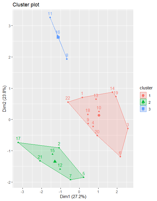
If there are more than two dimensions (variables) fviz_cluster will perform principal component analysis (PCA) and plot the data points according to the first two principal components that explain the majority of the variance.
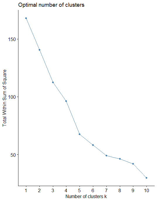
Optimal Clusters
We can find out optimal clusters in R with the following code. The results suggest that 4 is the optimal number of clusters as it appears to be the bend in the knee.
The same we executed above with traditional coding’s.
fviz_nbclust(nor, kmeans, method = "wss")
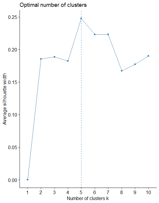
Average Silhouette Method
The average silhouette approach measures the quality of a clustering. It determines how well each observation lies within its cluster.
A high average silhouette width indicates a good clustering. The average silhouette method computes the average silhouette of observations for different values of k.
We can execute the same based on the below code
fviz_nbclust(nor, kmeans, method = "silhouette")
Gap Statistic Method
This approach can be utilized in any type of clustering method (i.e. K-means clustering, hierarchical clustering).
The gap statistic compares the total intracluster variation for different values of k with their expected values under null reference distribution of the data.
We can execute the same based on below code
gap_stat <- clusGap(nor, FUN = kmeans, nstart = 25,
                    K.max = 10, B = 50)
fviz_gap_stat(gap_stat)
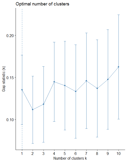
In this method also optimal number of cluster is 5.
Conclusion
K-means clustering is a very simple and fast algorithm and it can efficiently deal with very large data sets.
K-means clustering needs to provide a number of clusters as an input, Hierarchical clustering is an alternative approach that does not require that we commit to a particular choice of clusters.
Hierarchical clustering has an added advantage over K-means clustering because it has an attractive tree-based representation of the observations (dendrogram).

Hi, I am Sung, adjunct professor at SUNY Korea. I liked this post. Can I get your raw data? I cannot find the data. I would like to use it for my students. Thanks.
Hai, Data set available in the below link.
https://github.com/finnstats/finnstats
where can i found example dataset
Hai, You can get the data from the below link.
https://github.com/finnstats/finnstats