Random Forest Feature Selection

Random Forest feature selection, why we need feature selection?

When we have too many features or variables in the datasets and we want to develop a prediction model like a neural network will take a lot of computational time and more features reduce the accuracy of the prediction model. In such cases, we need to make use of the feature selection Boruta algorithm and which is based on a random forest.

How Boruta works?

Suppose if we have 100 variables in the dataset, each attributes creates shadow attributes, and in each shadow attribute, all the values are shuffled and creates randomness in the dataset.

Based on these datasets will create a classification model with shadow attributes and original attributes and then assess the importance of the attributes.

Random Forest Classification Model

Load Libraries

library(Boruta)
library(mlbench)
library(caret)
library(randomForest)

Getting Data

data("Sonar")
str(Sonar)

The dataset contains 208 observations with 61 variables.

'data.frame':     208 obs. of  61 variables:
 $ V1   : num  0.02 0.0453 0.0262 0.01 0.0762 0.0286 0.0317 0.0519 0.0223 0.0164 ...
 $ V2   : num  0.0371 0.0523 0.0582 0.0171 0.0666 0.0453 0.0956 0.0548 0.0375 0.0173 ...
 $ V3   : num  0.0428 0.0843 0.1099 0.0623 0.0481 ...
 $ V4   : num  0.0207 0.0689 0.1083 0.0205 0.0394 ...
 $ V5   : num  0.0954 0.1183 0.0974 0.0205 0.059 ...
 $ V6   : num  0.0986 0.2583 0.228 0.0368 0.0649 ...
 ...............................................
 $ V20  : num  0.48 0.782 0.862 0.397 0.464 ...
 $ V59  : num  0.009 0.0052 0.0095 0.004 0.0107 0.0051 0.0036 0.0048 0.0059 0.0056 ...
 $ V60  : num  0.0032 0.0044 0.0078 0.0117 0.0094 0.0062 0.0103 0.0053 0.0022 0.004 ...
 $ Class: Factor w/ 2 levels "M","R": 2 2 2 2 2 2 2 2 2 2 ...

Class is the dependent variable with 2 level factors Mine and Rock.

Market Basket Analysis in R

Feature Selection

set.seed(111)
boruta <- Boruta(Class ~ ., data = Sonar, doTrace = 2, maxRuns = 500)
print(boruta)

Boruta performed 499 iterations in 1.3 mins.

 33 attributes confirmed important: V1, V10, V11, V12, V13 and 28 more;
 20 attributes confirmed unimportant: V14, V24, V25, V29, V3 and 15 more;
 7 tentative attributes left: V2, V30, V32, V34, V39 and 2 more;

Based on Boruta algorithm 33 attributes are important, 20 attributes are unimportant and 7 are tentative attributes.

plot(boruta, las = 2, cex.axis = 0.7)

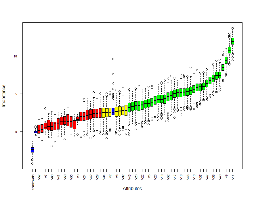
Blue box corresponds to shadow attributes, green color indicates important attributes, yellow boxes are tentative attributes and red boxes are unimportant.

plotImpHistory(boruta)

Tentative Fix

bor <- TentativeRoughFix(boruta)
print(bor)

Basically, TentativeRoughFix will take care of tentative attributes that are classified into really important or unimportant classes.

Decision Trees in R

Boruta performed 499 iterations in 1.3 mins.

Tentatives rough fixed over the last 499 iterations.
 35 attributes confirmed important: V1, V10, V11, V12, V13 and 30 more;
 25 attributes confirmed unimportant: V14, V2, V24, V25, V29 and 20 more;

attStats(boruta)

This will provide complete picture of all the variables.

meanImp medianImp  minImp maxImp normHits  decision
V1     3.63      3.66  1.0746    5.7    0.804 Confirmed
V2     2.54      2.55  0.0356    5.2    0.479 Tentative
V3     1.52      1.62 -0.4086    2.3    0.000  Rejected
V4     5.39      5.43  2.8836    8.4    0.990 Confirmed
V5     3.70      3.70  0.9761    5.9    0.814 Confirmed
V6     2.12      2.16 -0.4508    4.4    0.090  Rejected
V7     0.72      0.59 -0.4309    3.1    0.002  Rejected
V8     2.63      2.62 -0.3495    5.5    0.463 Tentative
.....................................................
V59    2.40      2.40 -0.5639    5.2    0.200  Rejected
V60    0.72      0.69 -1.9414    2.7    0.002  Rejected

Data Partition

Let’s partition the dataset into training datasets and test datasets. Now we want to build the Boruta algorithm for higher model accuracy.

set.seed(222)
ind <- sample(2, nrow(Sonar), replace = T, prob = c(0.6, 0.4))
train <- Sonar[ind==1,]
test <- Sonar[ind==2,]

Training dataset contains 117 observations and test data set contains 91 observations.

Cluster Analysis in R

Random Forest Model

set.seed(333) 
rf60 <- randomForest(Class~., data = train) 

Random forest model based on all the varaibles in the dataset

Call: randomForest(formula = Class ~ ., data = train)
               Type of random forest: classification
                     Number of trees: 500
No. of variables tried at each split: 7
        OOB estimate of  error rate: 23%
Confusion matrix:
   M  R class.error
M 51 10        0.16
R 17 39        0.30

OOB error rate is 23%

Prediction & Confusion Matrix – Test

p <- predict(rf60, test)
confusionMatrix(p, test$Class)

Confusion Matrix and Statistics

          Reference
Prediction  M  R
         M 46 17
         R  4 24
               Accuracy : 0.769        
                 95% CI : (0.669, 0.851)
    No Information Rate : 0.549        
    P-Value [Acc > NIR] : 1.13e-05     
                  Kappa : 0.52         
 Mcnemar's Test P-Value : 0.00883      
            Sensitivity : 0.920        
            Specificity : 0.585        
         Pos Pred Value : 0.730        \
         Neg Pred Value : 0.857        
             Prevalence : 0.549        
         Detection Rate : 0.505        
   Detection Prevalence : 0.692        
      Balanced Accuracy : 0.753        
       'Positive' Class : M    

Based on this model accuracy is around 76%. Now let’s make use of the Boruta model.

getNonRejectedFormula(boruta)
rfboruta <- randomForest(Class ~ V1 + V2 + V4 + V5 + V8 + V9 + V10 + V11 + V12 + V13 + 
                        V15 + V16 + V17 + V18 + V19 + V20 + V21 + V22 + V23 + V26 + 
                        V27 + V28 + V30 + V31 + V32 + V34 + V35 + V36 + V37 + V39 + 
                        V43 + V44 + V45 + V46 + V47 + V48 + V49 + V51 + V52 + V54, data = train)

Call: randomForest(formula = Class ~ V1 + V2 + V4 + V5 + V8 + V9 +      V10 + V11 + V12 + V13 + V15 + V16 + V17 + V18 + V19 + V20 +      V21 + V22 + V23 + V26 + V27 + V28 + V30 + V31 + V32 + V34 +      V35 + V36 + V37 + V39 + V43 + V44 + V45 + V46 + V47 + V48 +      V49 + V51 + V52 + V54, data = train)
               Type of random forest: classification
                     Number of trees: 500
No. of variables tried at each split: 6
        OOB estimate of  error rate: 22%
Confusion matrix:
   M  R class.error
M 52  9        0.15
R 17 39        0.30

Now you can see that the OOB error rate reduced from 23% to 22%.

p <- predict(rfboruta, test)
confusionMatrix(p, test$Class)

Confusion Matrix and Statistics

Linear Discriminant Analysis in R

          Reference
Prediction  M  R
         M 45 15
         R  5 26
               Accuracy : 0.78        
                 95% CI : (0.681, 0.86)
    No Information Rate : 0.549       
    P-Value [Acc > NIR] : 3.96e-06    
                  Kappa : 0.546       
 Mcnemar's Test P-Value : 0.0442      
            Sensitivity : 0.900       
            Specificity : 0.634       
         Pos Pred Value : 0.750       
         Neg Pred Value : 0.839       
             Prevalence : 0.549       
         Detection Rate : 0.495       
   Detection Prevalence : 0.659       
      Balanced Accuracy : 0.767       
       'Positive' Class : M 

Accuracy increased from 76% to 78%.

getConfirmedFormula(boruta)

rfconfirm <- randomForest(Class ~ V1 + V4 + V5 + V9 + V10 + V11 + V12 + V13 + V15 + V16 +
                            V17 + V18 + V19 + V20 + V21 + V22 + V23 + V26 + V27 + V28 +
                            V31 + V35 + V36 + V37 + V43 + V44 + V45 + V46 + V47 + V48 +
                            V49 + V51 + V52, data = train)

Call:

 randomForest(formula = Class ~ V1 + V4 + V5 + V9 + V10 + V11 +      V12 + V13 + V15 + V16 + V17 + V18 + V19 + V20 + V21 + V22 +      V23 + V26 + V27 + V28 + V31 + V35 + V36 + V37 + V43 + V44 +      V45 + V46 + V47 + V48 + V49 + V51 + V52, data = train)
               Type of random forest: classification
                     Number of trees: 500
No. of variables tried at each split: 5
        OOB estimate of  error rate: 20%
Confusion matrix:
   M  R class.error
M 53  8        0.13
R 15 41        0.27

Now you can see that based on important attributes is OOB error rate is further reduced into 20%.

Conclusion

Based on feature selection you can increase the accuracy of the model and if you are using neural network types of model can reduce the computational time also.

KNN Algorithm Machine Learning