Random Forest in R
Random Forest in R, Random forest developed by an aggregating tree and this can be used for classification and regression. One of the major advantages is its avoids overfitting.
The random forest can deal with a large number of features and it helps to identify the important attributes.
The random forest contains two user-friendly parameters ntree and mtry.
ntree- ntree by default is 500 trees.
mtry- variables randomly samples as candidates at each split.
Random Forest Steps
1. Draw ntree bootstrap samples.
2. For each bootstrap, grow an un-pruned tree by choosing the best split based on a random sample of mtry predictors at each node
3. Predict new data using majority votes for classification and average for regression based on ntree trees.
Load Library
library(randomForest)
library(datasets)
library(caret)
Getting Data
data<-iris
str(data)
The datasets contain 150 observations and 5 variables. Species considered as response variables. Species variable should be a factor variable.
data$Species <- as.factor(data$Species)
table(data$Species)
setosa versicolor  virginica
 50         50         50
From the above results, we can identify that our data set is balanced.
Data Partition
Lets start with random seed so the outcome will be repeatable and store train and test data.
set.seed(222)
ind <- sample(2, nrow(data), replace = TRUE, prob = c(0.7, 0.3))
train <- data[ind==1,]
test <- data[ind==2,]
106 observations in train data set and 44 observatons in test data.
Random Forest in R
rf <- randomForest(Species~., data=train, proximity=TRUE) print(rf)
Call:
 randomForest(formula = Species ~ ., data = train)
               Type of random forest: classification
                     Number of trees: 500
No. of variables tried at each split: 2
        OOB estimate of  error rate: 2.83%
Confusion matrix:
           setosa versicolor virginica class.error
setosa         35          0         0  0.00000000
versicolor      0         35         1  0.02777778
virginica       0          2        33  0.05714286
Out of bag error is 2.83%, so the train data set model accuracy is around 97%.
Ntree is 500 and mtry is 2
Prediction & Confusion Matrix – train data
p1 <- predict(rf, train)
confusionMatrix(p1, train$ Species)
Confusion Matrix and Statistics
            Reference
Prediction   setosa versicolor virginica
  setosa         35          0         0
  versicolor      0         36         0
  virginica       0          0        35
Overall Statistics
               Accuracy : 1
                 95% CI : (0.9658, 1)
    No Information Rate : 0.3396
    P-Value [Acc > NIR] : < 2.2e-16
                  Kappa : 1
 Mcnemar's Test P-Value : NA
Statistics by Class:
                     Class: setosa Class: versicolor Class: virginica
Sensitivity                 1.0000            1.0000           1.0000
Specificity                 1.0000            1.0000           1.0000
Pos Pred Value              1.0000            1.0000           1.0000
Neg Pred Value              1.0000            1.0000           1.0000
Prevalence                  0.3302            0.3396           0.3302
Detection Rate              0.3302            0.3396           0.3302
Detection Prevalence        0.3302            0.3396           0.3302
Balanced Accuracy           1.0000            1.0000           1.0000
Train data accuracy is 100% that indicates all the values classified correctly.
Naive Bayes Classification in R
Prediction & Confusion Matrix – test data
p2 <- predict(rf, test)
confusionMatrix(p2, test$ Species)
Confusion Matrix and Statistics
            Reference
Prediction   setosa versicolor virginica
  setosa         15          0         0
  versicolor      0         11         1
  virginica       0          3        14
Overall Statistics
               Accuracy : 0.9091
                 95% CI : (0.7833, 0.9747)
    No Information Rate : 0.3409
-    P-Value [Acc > NIR] : 5.448e-15
                  Kappa : 0.8634
 Mcnemar's Test P-Value : NA
Statistics by Class:
                     Class: setosa Class: versicolor Class: virginica
Sensitivity                 1.0000            0.7857           0.9333
Specificity                 1.0000            0.9667           0.8966
Pos Pred Value              1.0000            0.9167           0.8235
Neg Pred Value              1.0000            0.9062           0.9630
Prevalence                  0.3409            0.3182           0.3409
Detection Rate              0.3409            0.2500           0.3182
Detection Prevalence        0.3409            0.2727           0.3864
Balanced Accuracy           1.0000            0.8762           0.9149
Test data accuracy is 90%
Error rate of Random Forest
plot(rf)
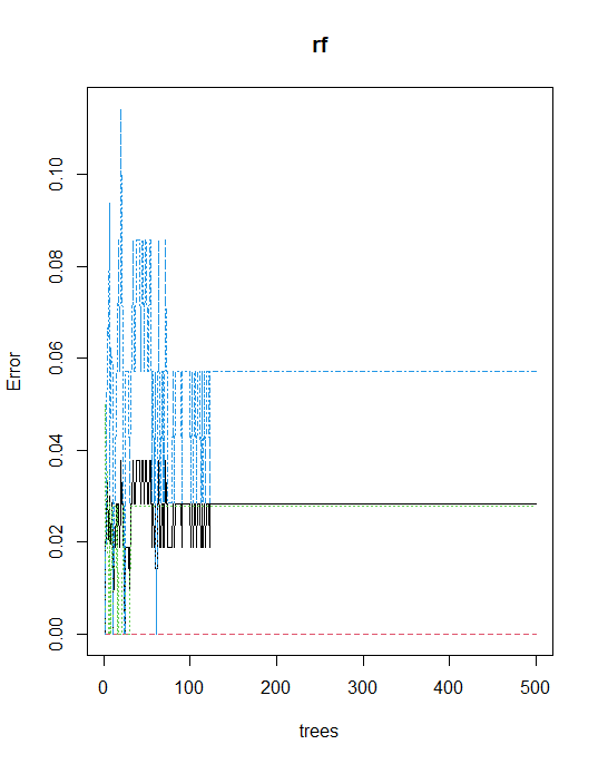
The model is predicted with high accuracy, with no need for further tuning. However, we can tune a number of trees and mtry basis below the function.
Tune mtry
t <- tuneRF(train[,-5], train[,5],
       stepFactor = 0.5,
       plot = TRUE,
       ntreeTry = 150,
       trace = TRUE,
       improve = 0.05)
No. of nodes for the trees
hist(treesize(rf),
     main = "No. of Nodes for the Trees",
     col = "green")
Variable Importance
varImpPlot(rf,
           sort = T,
           n.var = 10,
           main = "Top 10 - Variable Importance")
importance(rf)
MeanDecreaseGini
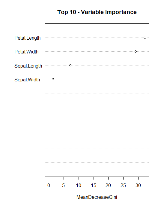
Sepal.Length         7.170376
Sepal.Width          1.318423
Petal.Length        32.286286
Petal.Width         29.117348
Petal.Length is the most important attribute followed by Petal.Width.
Partial Dependence Plot
partialPlot(rf, train, Petal.Width, "setosa")
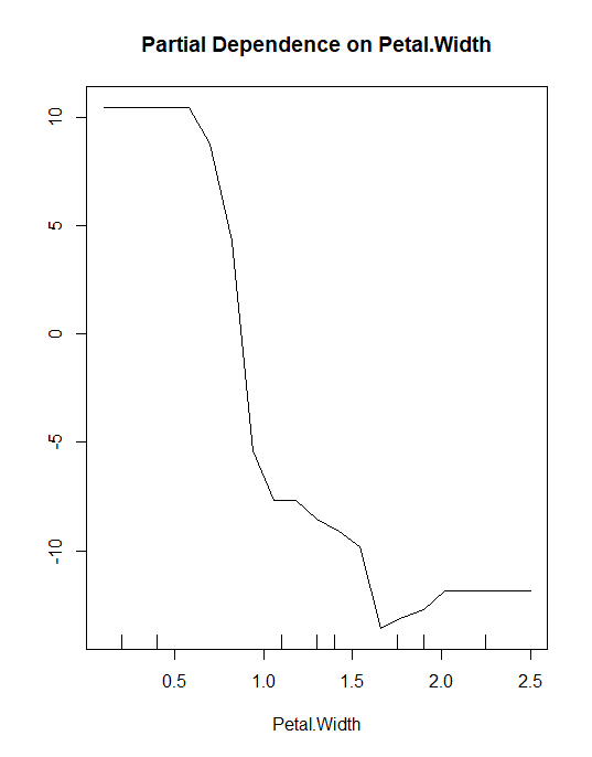
The inference should be, if the petal width is less than 1.5 then higher chances of classifying into Setosa class.
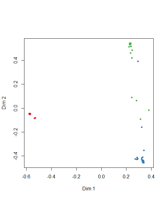
Multi-dimensional Scaling Plot of Proximity Matrix
Dimension plot also can create from random forest model.
MDSplot(rf, train$Species)


I worked through your tutorial with another dataset and experienced that the factor column needed to be the last column. Thanks for the tutorial
Yes, I took the response variable as the last column. Thanks for your reply…