Handling missing values in R
Handling missing values in R, one of the common tasks in data analysis is handling missing values.
In R, missing values are often represented by the symbol NA (not available) or some other value that represents missing values (i.e. 99).
Impossible values (e.g., dividing by zero) are represented by the symbol NaN (not a number)
Handling missing values in R
You can test the missing values based on the below command in R
y <- c(1,2,3,NA)
is.na(y) # returns a vector (F F F T)
This function you can use for vector as well as data frame also.
To identify the location of NAs in a vector, you can use which command.
which(is.na(y))
In the case of data frame, sum function will be handy
sum(is.na(df))
df indicates the data frame
the function will return a total number of NA values.
In the case of data frames with multiple columns, a convenient shortcut method is colSum.
colSums(is.na(df))
the summary function also can be used for finding missing values in data frames.
Suppose if you are calculating the average value then na.rm will be very useful.
x[is.na(x)] <- mean(x, na.rm = TRUE)
Sometimes values are stored as 99 that you can convert into NA using the following command.
df$v1[df$v1==99] <- NA
one of the common methods is na.omit.
The function na.omit() returns the object with listwise deletion of missing values
This function create new dataset without missing data
newdata <- na.omit(df)
Another traditional way of handling missing value is based on complele.cases.
The function complete.cases() returns a logical vector indicating which cases are complete.
This will list rows of data that have missing values
df[!complete.cases(df),]
subset with complete.cases to get complete cases
df[complete.cases(df), ]
Deleting rows containing missing values, lead to a reduction in sample size and avoid some good representative values also.
Delete Missing Data leads to the following major issues
- Data loss
- Bias data
Above mentioned methods are not handy in some cases, one of the commonly used method is to replace NA values based on average. In some cases this will be erroneous.
Imagine supposing if we have vehicle failure data with the following details
| Vehicle | Month | Distance Travelled |
| 1 | 35 | 20000 |
| 2 | 24 | 18000 |
| 3 | 1 | NA |
| 4 | 12 | 6000 |
In the above data if we are replacing NA values with 14666 (ie. average value) will be erroneous because just a one-month-old vehicle traveled this much distance is unlikely.
Now here we are going to discuss, how to deal with this kind of issue smartly!
Load Libraries
library(mice)
library(VIM)
Getting Data
data <- read.csv("D:/RStudio/MissingDataAnalysis/VehicleData.csv", header = T)
str(data)
'data.frame': 1624 obs. of 7 variables: $ vehicle: int 1 2 3 4 5 6 7 8 9 10 ... $ fm : int 0 10 15 0 13 21 11 5 8 1 ... $ Mileage: int 863 4644 16330 13 22537 40931 34762 11051 7003 11 ... $ lh : num 1.1 2.4 4.2 1 4.5 3.1 0.7 2.9 3.4 0.7 ... $ lc : num 66.3 233 325.1 66.6 328.7 ... $ mc : num 697 120 175 0 175 ... $ State : chr "MS" "CA" "WI" "OR" ...
In this dataset contains 1624 observations and 7 variables. You can access data set from here.
summary(data)
vehicle             fm            Mileage            lh               lc               mc            State
Min.   :   1.0   Min.   :-1.000   Min.   :    1   Min.   : 0.000   Min.   :   0.0   Min.   :   0.0   Length:1624
1st Qu.: 406.8   1st Qu.: 4.000   1st Qu.: 5778   1st Qu.: 1.500   1st Qu.: 106.5   1st Qu.: 119.7   Class :character
Median : 812.5   Median :10.000   Median :17000   Median : 2.600   Median : 195.4   Median : 119.7   Mode  :character
Mean   : 812.5   Mean   : 9.414   Mean   :20559   Mean   : 3.294   Mean   : 242.8   Mean   : 179.4
3rd Qu.:1218.2   3rd Qu.:14.000   3rd Qu.:30061   3rd Qu.: 4.300   3rd Qu.: 317.8   3rd Qu.: 175.5
Max.   :1624.0   Max.   :23.000   Max.   :99983   Max.   :35.200   Max.   :3234.4   Max.   :3891.1
NA's   :13      NA's   :6        NA's   :8
Based on summary function as mentioned earlier we can find out the details of column contains missing values.
Missing data
Now we need to calculate what percentage of data is missing from each variable.
p <- function(x) {sum(is.na(x))/length(x)*100}
apply(data, 2, p)
vehicle fm Mileage lh lc mc State 0.0 0.0000000 0.8004926 0.3694581 0.4926108 0.0000000 0.9236453
Vehicle, fm and mc contains no missing values, lh contains 0.36%, lc contains 0.49%, Mileage contains 0.80% and maximum missing in state column with 0.92%
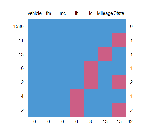
md.pattern(data)

     vehicle fm mc lh lc   Mileage State
1586       1  1  1  1  1       1     1  0
11         1  1  1  1  1       1     0  1
13         1  1  1  1  1       0     1  1
6          1  1  1  1  0       1     1  1
2          1  1  1  1  0       1     0  2
4          1  1  1  0  1       1     1  1
2          1  1  1  0  1       1     0  2
           0  0  0  6  8      13    15 42
zero indicates missing values, for example column ‘state’ contains 11 rows with one missing values.
Similarly, 13 rows mileage values are missing.
md.pairs(data)
$rr
        vehicle   fm Mileage   lh   lc   mc State
vehicle    1624 1624    1611 1618 1616 1624  1609
fm         1624 1624    1611 1618 1616 1624  1609
Mileage    1611 1611    1611 1605 1603 1611  1596
lh         1618 1618    1605 1618 1610 1618  1605
lc         1616 1616    1603 1610 1616 1616  1603
mc         1624 1624    1611 1618 1616 1624  1609
State      1609 1609    1596 1605 1603 1609  1609
$rm
        vehicle fm Mileage lh lc mc State
vehicle       0  0      13  6  8  0    15

fm            0  0      13  6  8  0    15
Mileage       0  0       0  6  8  0    15
lh            0  0      13  0  8  0    13
lc            0  0      13  6  0  0    13
mc            0  0      13  6  8  0    15
State         0  0      13  4  6  0     0
$mr
        vehicle fm Mileage lh lc mc State
vehicle       0  0       0  0  0  0     0
fm            0  0       0  0  0  0     0
Mileage      13 13       0 13 13 13    13
lh            6  6       6  0  6  6     4
c            8  8       8  8  0  8     6
mc            0  0       0  0  0  0     0
State        15 15      15 13 13 15     0
$mm
        vehicle fm Mileage lh lc mc State
vehicle       0  0       0  0  0  0     0
fm            0  0       0  0  0  0     0
Mileage       0  0      13  0  0  0     0
lh            0  0       0  6  0  0     2
lc            0  0       0  0  8  0     2
mc            0  0       0  0  0  0     0
State         0  0       0  2  2  0    15
rr indicates how many data points are observed
rm indicates Observed and Missing
mr indicates Mossing versus observed
mm indicates Missing versus Missing
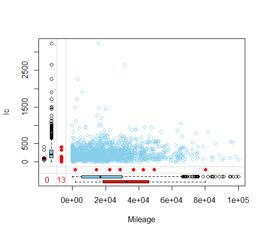
marginplot(data[,c('Mileage', 'lc')])
Blue values are observed values and red ones are missing values.
Impute
impute <- mice(data[,2:7], m=3, seed = 123)
print(impute)
Class: mids
Number of multiple imputations:  3
Imputation methods:
     fm Mileage      lh      lc      mc   State
     ""   "pmm"   "pmm"   "pmm"      ""      ""
PredictorMatrix:
        fm Mileage lh lc mc State
fm       0       1  1  1  1     0
Mileage  1       0  1  1  1     0
lh       1       1  0  1  1     0
lc       1       1  1  0  1     0
mc       1       1  1  1  0     0
State    0       0  0  0  0     0
Number of logged events:  1
  it im dep     meth   out
1  0  0     constant State
Here you can see different methods for imputation.
For example, variable fm contains no missing values and hence no method applied.
For the variable Mileage, lh and lc “pmm” method used.
pmm stands for predictive Mean Matching.
polyreg used for factor variables, polyreg stands for multinomial logistic regression.
impute$imp$Mileage
   1     2     3
19   40558 25481 21179
20   25478 13785 16319
253    138  1945   251
254  13089 16963 31078
255  26785 47232 22101
256  34822 33543 19486
861   6136 17212 75106
862   2844   243  1591
863  16319 19539 17610
1568 29262 17948 27095
1569 15299 11912  3253
1570    94   277    31
1571  3296 11000 17217
Total 3 imputations calculated here for understanding purpose, the best imputation value suited to your dataset can used for further analysis. Just look at the 20th row
data[20,]
vehicle fm Mileage  lh    lc   mc State
20      20  8      NA 1.4 87.42 1.85    NH
20th-row Mileage is missing the first imputation is represent is 25478, the second one is 13785, and the third one is 16319. So ideally the all values are always better than average.
Complete data
newDATA <- complete(impute, 1)
Distribution of oberserved/imputed values
xyplot(impute, lc ~ lh | .imp, pch = 20, cex=1.4)

First, one is original observations and followed by impute1, 2, and 3. You can see there are no changes after imputing the observations.
Conclusion
Based on the mice package missing values can handle smartly, understand your data sets, and apply correct algorithms.
If you are using any other methods or functions please mention in comments section.


Hi –
Thanks for this tutorial. Can you please explain how to get to the VehicleData file? I don’t have a D drive on my computer (Windows 10). The code you provide is:
read.csv(“D:/RStudio/MissingDataAnalysis/VehicleData.csv”, header = T)
I get an error message because it can’t find my D drive – and I don’t know how the file would have gotten in there in the first place. Can you please explain. Thank you very much!
Jean
Hai Jean,
Vehicle data were available in the below link. You can save the data in excel format and can change the script read.csv file location accordingly.
https://github.com/finnstats/finnstats/blob/main/VehicleData.csv