Linear Discriminant Analysis in R, originally developed by R A Fisher in 1936 to classify subjects into one of the two clearly defined groups.

It was later expanded to classify subjects into more than two groups.

Linear Discriminant Analysis (LDA) is a dimensionality reduction technique. LDA used for dimensionality reduction to reduce the number of dimensions (i.e. variables) in a dataset while retaining as much information as possible.

Basically, it helps to find the linear combination of original variables that provide the best possible separation between the groups.

Customer Segmentation analysis in R

The basic purpose is to estimate the relationship between a single categorical dependent variable and a set of quantitative independent variables.

The major applications or examples are

• Predicting success or failure of new products
• Accepting or rejecting admission to an applicant.
• Predicting credit risk category for a person
• Classifying patients into different categories.

Let’s look into the iris data set for further analysis.

Regression analysis in R

Load Library

library(klaR)
library(psych)
library(MASS)
library(ggord)
library(devtools)

Getting Data

data("iris")
str(iris)

Total 150 observations and 5 variables contains in the iris dataset.

'data.frame':       150 obs. of  5 variables:
 $ Sepal.Length: num  5.1 4.9 4.7 4.6 5 5.4 4.6 5 4.4 4.9 ...
 $ Sepal.Width : num  3.5 3 3.2 3.1 3.6 3.9 3.4 3.4 2.9 3.1 ...
 $ Petal.Length: num  1.4 1.4 1.3 1.5 1.4 1.7 1.4 1.5 1.4 1.5 ...
 $ Petal.Width : num  0.2 0.2 0.2 0.2 0.2 0.4 0.3 0.2 0.2 0.1 ...
 $ Species     : Factor w/ 3 levels "setosa","versicolor",..: 1 1 1 1 1 1 1 1 1 1 ...

First will create a scatterplot for the first four numerical variables. The gap between the points given is zero.

Social Network Analysis in R

pairs.panels(iris[1:4],
             gap = 0,
             bg = c("red", "green", "blue")[iris$Species],
             pch = 21)

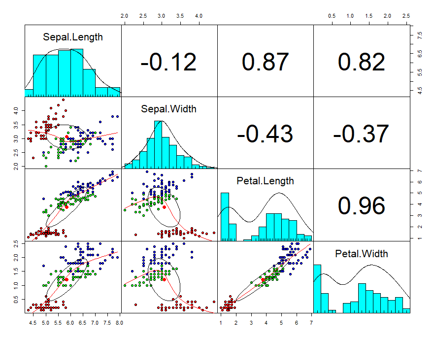
Now you can see in the plot, scatter diagram, histogram, and correlation values.

Now we want to create the best separation groups based on these species.

Data partition

Let’s create a training dataset and test dataset for prediction and testing purposes. 60% dataset used for training purposes and 40$ used for testing purposes.

set.seed(123)
ind <- sample(2, nrow(iris),
              replace = TRUE,
              prob = c(0.6, 0.4))
training <- iris[ind==1,]
testing <- iris[ind==2,]

Linear discriminant analysis

linear <- lda(Species~., training)
linear

Call:

lda(Species ~ ., data = training)
Prior probabilities of groups:
    setosa versicolor  virginica
 0.3837209  0.3139535  0.3023256
Group means:
           Sepal.Length Sepal.Width Petal.Length Petal.Width
setosa         4.975758    3.357576     1.472727   0.2454545
versicolor     5.974074    2.751852     4.281481   1.3407407
virginica      6.580769    2.946154     5.553846   1.9807692
Coefficients of linear discriminants:
                   LD1        LD2
Sepal.Length  1.252207 -0.1229923
Sepal.Width   1.115823  2.2711963
Petal.Length -2.616277 -0.7924520
Petal.Width  -2.156489  2.6956343
The proportion of trace:
   LD1    LD2
0.9937 0.0063

Based on the training dataset, 38% belongs to setosa group, 31% belongs to versicolor groups and 30% belongs to virginica groups.

Decision Trees in R

The first discriminant function is a linear combination of the four variables.

Percentage separations achieved by the first discriminant function is 99.37% and second is 0.63%

attributes(linear)

[1] "prior"   "counts"  "means"   "scaling" "lev"     "svd"     "N"       "call"    "terms" 
[10] "xlevels"
$class
[1] "lda"

Histogram

Stacked histogram for discriminant function values.

p <- predict(linear, training)
ldahist(data = p$x[,1], g = training$Species)

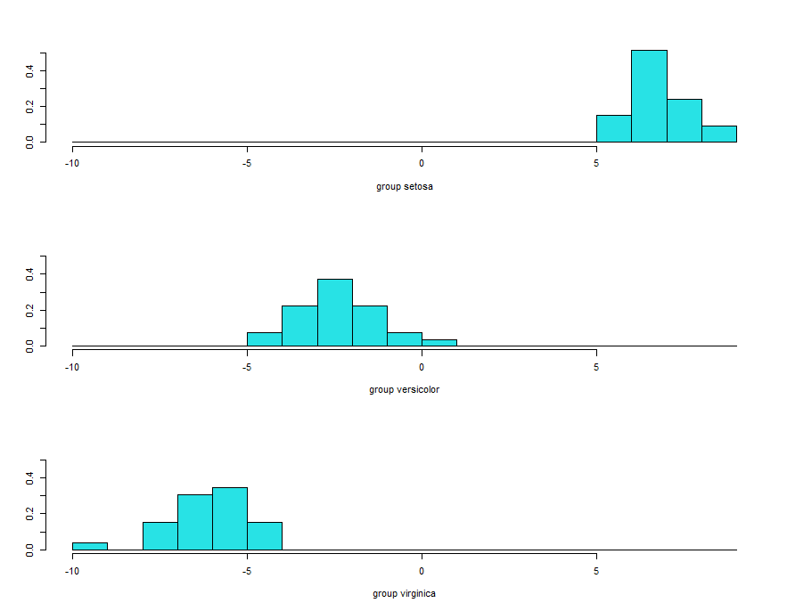
These histograms are based on ld1. It’s clearly evident that no overlaps between first and second and first and third species. But some overlap observed between the second and third species.

Market Basket Analysis in R

ldahist(data = p$x[,2], g = training$Species)

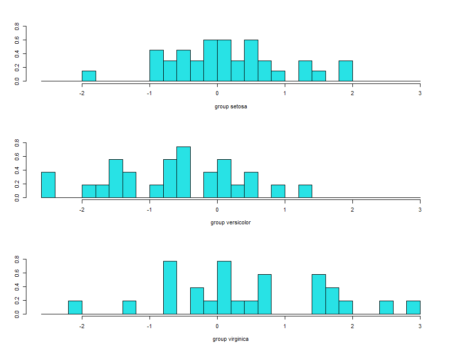
histogram based on lda2 showing complete overlap and its not good.

Bi-Plot

ggord(linear, training$Species, ylim = c(-10, 10))

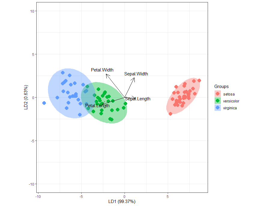
Biplot based on LD1  and LD2. Setosa separated very clearly and some overlap observed between Versicolor and virginica.

Based on arrows, Sepal width and sepal length explained more for setosa, petal width and petal length explained more for versicolor and virginica.

Deep Neural Network in R

Partition plot

It provides the classification of each and every combination in the training dataset.

partimat(Species~., data = training, method = "lda")

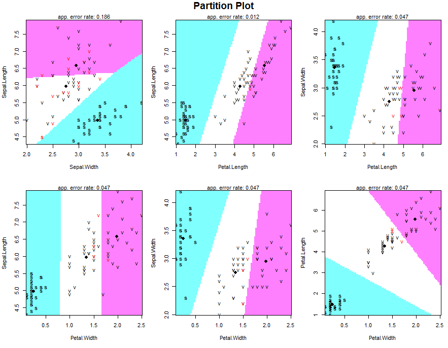
partimat(Species~., data = training, method = "qda")

Confusion matrix and accuracy – training data

p1 <- predict(linear, training)$class
tab <- table(Predicted = p1, Actual = training$Species)
tab

Let’s see the correct classifications and miss classifications.

Repeated Measures of ANOVA in R

Actual
Predicted    setosa versicolor virginica
  setosa         33          0         0
  versicolor      0         26         1
  virginica       0          1        25

In the training dataset total correct classification is 33+26+25=84

sum(diag(tab))/sum(tab)

The accuracy of the model is around 0.9767442

Confusion matrix and accuracy – testing data

p2 <- predict(linear, testing)$class
tab1 <- table(Predicted = p2, Actual = testing$Species)
tab1

Actual
Predicted    setosa versicolor virginica
  setosa         17          0         0
  versicolor      0         22         0
  virginica       0          1        24

sum(diag(tab1))/sum(tab1)

The accuracy of the model is around .984375

Conclusion

Histogram and Biplot provide useful insights and helpful for interpretations and if there is not a great difference in the group covariance matrices, then the linear discriminant analysis will perform as well as quadratic. LDA is not useful for solving non-linear problems.

KNN Algorithm Machine Learning