Stock Price Prediction in R: A Complete Guide Using Statistical Models and Machine Learning
Stock Price Prediction in R, Predicting stock prices has long been one of the most challenging and fascinating problems in finance. Investors, hedge funds, quantitative analysts, and fintech companies continuously seek methods to forecast market movements and identify profitable investment opportunities.
With the growth of big data, artificial intelligence, and machine learning, stock price prediction has evolved far beyond traditional chart analysis. Modern forecasting techniques leverage historical price data, technical indicators, statistical models, and machine learning algorithms to uncover patterns that may help predict future market behavior.
R provides a powerful ecosystem for financial analytics, time series forecasting, statistical modeling, and machine learning, making it one of the preferred tools for quantitative finance professionals.
This guide explores stock price prediction in R using practical examples, forecasting models, machine learning techniques, and best practices.
What Is Stock Price Prediction in R?
Stock price prediction refers to estimating future stock prices or returns using historical market data and predictive models.
Common prediction targets include:
- Next-day stock price
- Future returns
- Market direction
- Volatility forecasting
- Trend prediction
- Buy and sell signals
The goal is not necessarily to predict exact prices but to improve investment decisions using data-driven insights.
Why Use R for Stock Price Prediction?
R offers several advantages:
Advanced Statistical Modeling
R was built specifically for statistical analysis and forecasting.
Financial Analytics Libraries
Popular packages include:
- quantmod
- forecast
- TTR
- PerformanceAnalytics
- xts
- zoo
Machine Learning Support
R supports:
- Random Forest
- XGBoost
- Neural Networks
- Support Vector Machines
- Deep Learning
Data Visualization
Powerful charting capabilities help identify trends and patterns.
Installing Required Packages
install.packages(c(
  "quantmod",
  "forecast",
  "TTR",
  "PerformanceAnalytics",
  "caret",
  "randomForest",
  "xts"
))
Load libraries:
library(quantmod)
library(forecast)
library(TTR)
library(PerformanceAnalytics)
library(caret)
library(randomForest)
library(xts)
Downloading Stock Market Data
We’ll use Apple stock data from Yahoo Finance.
library(quantmod)

getSymbols(
  "AAPL",
  src = "yahoo",
  from = "2020-01-01"
)

head(AAPL)
The dataset includes:
- Open
- High
- Low
- Close
- Volume
- Adjusted Close
Visualizing Stock Prices
chartSeries(
  AAPL,
  theme = chartTheme("white")
)
Visual exploration often reveals:
- Trends
- Volatility
- Price cycles
- Market shocks
Creating Daily Returns
Returns are often easier to model than raw prices.
returns <- dailyReturn(
  Ad(AAPL)
)

head(returns)
Visualize returns:
hist(
  returns,
  breaks = 50,
  main = "Distribution of Daily Returns"
)
Moving Average Forecasting
Moving averages help smooth price fluctuations.
Calculate Moving Averages
AAPL$SMA20 <- SMA(
  Cl(AAPL),
  n = 20
)

AAPL$SMA50 <- SMA(
  Cl(AAPL),
  n = 50
)
Plot:
chartSeries(
  AAPL,
  TA = c(
    addSMA(20),
    addSMA(50)
  )
)
These indicators are frequently used in trading systems.
Time Series Forecasting Using ARIMA
ARIMA remains one of the most widely used forecasting techniques.
Build ARIMA Model
price <- Ad(AAPL)

fit <- auto.arima(price)
Model summary:
summary(fit)
Forecast next 30 days:
future <- forecast(
  fit,
  h = 30
)

plot(future)
ARIMA is useful for capturing trends and autocorrelation patterns.
Exponential Smoothing Forecast
Another popular forecasting approach:
ets_model <- ets(price)

ets_forecast <- forecast(
  ets_model,
  h = 30
)

plot(ets_forecast)
Exponential smoothing often performs well for stable time series.
Feature Engineering for Machine Learning
Machine learning models require predictor variables.
Create technical indicators:
data <- data.frame(
  Close = as.numeric(
    Cl(AAPL)
  )
)

data$RSI <- RSI(
  Cl(AAPL),
  n = 14
)

data$SMA20 <- SMA(
  Cl(AAPL),
  n = 20
)

data$SMA50 <- SMA(
  Cl(AAPL),
  n = 50
)

data$Volume <- as.numeric(
  Vo(AAPL)
)
Remove missing values:
data <- na.omit(data)
Creating Prediction Target
Predict tomorrow’s closing price:
data$Target <-
  dplyr::lead(
    data$Close,
    1
  )

data <- na.omit(data)
Train-Test Split
set.seed(123)

train_index <- createDataPartition(
  data$Target,
  p = 0.8,
  list = FALSE
)

train <- data[
  train_index,
]

test <- data[
  -train_index,
]
Random Forest Stock Prediction
Random Forest is one of the most popular machine learning algorithms in finance.
rf_model <- randomForest(
  Target ~ .,
  data = train,
  ntree = 500
)
Generate predictions:
predictions <- predict(
  rf_model,
  newdata = test
)
Evaluate accuracy:
RMSE(
  predictions,
  test$Target
)
Feature Importance Analysis
Identify which indicators contribute most to predictions.
importance(
  rf_model
)
Plot importance:
varImpPlot(
  rf_model
)
This helps explain model behavior.
Predicting Market Direction
Instead of forecasting exact prices, many traders predict direction.
Create binary target:
data$Direction <- ifelse(
  data$Target >
  data$Close,
  "UP",
  "DOWN"
)
Train classification model:
rf_direction <- randomForest(
  as.factor(Direction) ~
    RSI +
    SMA20 +
    SMA50 +
    Volume,
  data = train
)
Predict:
predict(
  rf_direction,
  newdata = test
)
Model Evaluation
Key metrics include:
RMSE
sqrt(
  mean(
    (
      predictions -
      test$Target
    )^2
  )
)
MAE
mean(
  abs(
    predictions -
    test$Target
  )
)
Accuracy
For classification models:
confusionMatrix(
  predicted,
  actual
)
Advanced Machine Learning Models
Professional quantitative investors often use:
XGBoost
High-performance gradient boosting.
Neural Networks
Capture nonlinear market relationships.
LSTM Networks
Designed for sequential time series data.
Transformers
Increasingly used in financial forecasting.
Ensemble Models
Combine multiple forecasting techniques.
Challenges of Stock Price Prediction
Predicting markets is difficult because of:
Market Efficiency
Public information is quickly reflected in prices.
Unexpected Events
News, earnings, and economic shocks create sudden movements.
Non-Stationary Data
Market behavior changes over time.
Overfitting
Models may perform well historically but fail in live trading.
Best Practices
- Use adjusted prices.
- Incorporate technical indicators.
- Test multiple models.
- Avoid look-ahead bias.
- Perform out-of-sample validation.
- Consider transaction costs.
- Continuously retrain models.
- Focus on risk-adjusted performance.
Real-World Applications
Stock price prediction is widely used by:
Hedge Funds
Develop quantitative trading strategies.
Investment Banks
Forecast asset prices and risk.
FinTech Companies
Power robo-advisors and trading platforms.
Asset Managers
Support investment decisions.
Retail Traders
Generate trading signals.
Conclusion
Stock price prediction in R combines financial analytics, statistical modeling, and machine learning to uncover patterns within market data. While no model can perfectly predict future stock prices, data-driven approaches can improve decision-making, enhance risk management, and support systematic investment strategies.
By leveraging R’s rich ecosystem of financial and machine learning packages, analysts and investors can build forecasting models ranging from simple moving averages and ARIMA models to advanced Random Forests, XGBoost systems, and deep learning architectures. As AI and quantitative finance continue to evolve, stock price prediction remains one of the most valuable applications of data science in modern investing.