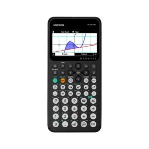
Poisson Probabilities on TI-84 Calculator
Poisson Probabilities on TI-84 Calculator, The Poisson distribution is a discrete probability distribution used to model the number of times an event occurs within a fixed interval of time, distance, area, volume, or another specified unit. It is especially useful when events occur independently and at a relatively constant average rate.
For example, Poisson probabilities can be used to study:
- The number of customer arrivals per hour
- The number of emails received per minute
- The number of defects in a production batch
- The number of calls received by a support center
- The number of website visitors during a given time period
- The number of accidents occurring at an intersection during a month
The TI-84 calculator has built-in functions that make it easy to calculate both individual and cumulative Poisson probabilities.
What Is the Poisson Distribution?
A random variable X follows a Poisson distribution when it represents the number of events occurring during a fixed interval and the events occur independently at a constant average rate.
The Poisson distribution has one primary parameter:
λ (lambda) = the average number of events occurring within the specified interval.
The probability of observing exactly x events is given by: P(X=x)=e−λ λx/x!
where:
- X = number of events
- x = specific number of events
- λ = average number of events
- e ≈ 2.71828
- x! = factorial of x
For a Poisson random variable: μ=λ
and σ=λ
Therefore, if the average number of events is 9, the mean is 9 and the standard deviation is 3.
Poisson PDF vs. Poisson CDF
The TI-84 provides two important Poisson functions:
poissonpdf()
The poissonpdf( function calculates the probability of exactly x events.
The syntax is:
poissonpdf(λ, x)
For example:
poissonpdf(4, 3)
calculates: P(X=3)
when the average number of events is 4.
poissoncdf()
The poissoncdf( function calculates the probability of observing x or fewer events.
The syntax is:
poissoncdf(λ, x)
For example:
poissoncdf(4, 3)
calculates: P(X≤3)
which includes the probabilities of observing 0, 1, 2, or 3 events.
How to Access Poisson Functions on a TI-84
To access the Poisson probability functions:
- Turn on your TI-84 calculator.
- Press 2nd.
- Press VARS to open the
DISTRmenu. - Scroll down to find
poissonpdf(orpoissoncdf(. - Press ENTER.
You can then enter the required parameters.
Example 1: Probability of Exactly 3 Events
Suppose a help desk receives an average of 4 emails per hour. What is the probability that exactly 3 emails will be received during the next hour?
Here: λ=4
and x=3
Because we want the probability of exactly 3 events, use poissonpdf(.
On the TI-84, enter:
poissonpdf(4,3)
The result is approximately: P(X=3)=0.1954
Therefore, there is approximately a 19.54% probability that exactly 3 emails will be received during the hour.
Example 2: Probability of 3 or Fewer Events
Using the same example, suppose you want to determine the probability that the help desk receives 3 or fewer emails during the hour.
Now we need: P(X≤3)
Use the poissoncdf( function:
poissoncdf(4,3)
The result is approximately: P(X≤3)=0.4335
Therefore, there is approximately a 43.35% probability that the help desk receives 3 or fewer emails during the hour.
Example 3: Probability of More Than 3 Events
Suppose you want to find the probability that the help desk receives more than 3 emails.
This can be calculated using the complement: P(X>3)=1−P(X≤3)
From the previous example: P(X≤3)=0.4335
Therefore: P(X>3)=1−0.4335 P(X>3)≈0.5665
On the TI-84, you can enter:
1-poissoncdf(4,3)
The result is approximately: 0.5665
So there is approximately a 56.65% probability of receiving more than 3 emails during the hour.
Example 4: Probability of At Least 5 Events
Suppose a website receives an average of 6 customer inquiries per day. What is the probability of receiving at least 5 inquiries tomorrow?
Here: λ=6
We want: P(X≥5)
Because poissoncdf() calculates the probability of X≤x, use the complement: P(X≥5)=1−P(X≤4)
On the TI-84, enter:
1-poissoncdf(6,4)
This gives the probability of receiving at least 5 inquiries.
Example 5: Probability Between Two Values
Suppose a manufacturing process produces an average of 8 defects per week. What is the probability that between 5 and 10 defects, inclusive, occur in a particular week?
We want: P(5≤X≤10)
This can be calculated using: P(X≤10)−P(X≤4)
On the TI-84, enter:
poissoncdf(8,10)-poissoncdf(8,4)
This gives the probability of observing between 5 and 10 defects, inclusive.
Understanding Common Poisson Probability Questions
The wording of a probability question determines which calculation you need.
| Question | Mathematical Form | TI-84 Approach |
|---|---|---|
| Exactly 5 events | P(X=5) | poissonpdf(λ,5) |
| 5 or fewer | P(X≤5) | poissoncdf(λ,5) |
| Fewer than 5 | P(X<5) | poissoncdf(λ,4) |
| More than 5 | P(X>5) | 1-poissoncdf(λ,5) |
| At least 5 | P(X≥5) | 1-poissoncdf(λ,4) |
| Between 5 and 10 inclusive | P(5≤X≤10) | poissoncdf(λ,10)-poissoncdf(λ,4) |
This distinction is particularly important because “at least,” “more than,” “fewer than,” and “at most” correspond to different inequalities.
Changing the Time Interval
The value of λ must correspond to the interval being analyzed.
For example, suppose a call center receives an average of 12 calls per hour. If you want to calculate the probability of calls during a 30-minute period, you cannot simply use λ = 12.
Because 30 minutes is half an hour: λ=12(0.5)=6
Therefore, the appropriate Poisson model for the 30-minute period has: λ=6
Similarly, for a two-hour period: λ=12(2)=24
Correctly adjusting λ for the time or space interval is essential when applying the Poisson distribution.
Conditions for Using a Poisson Distribution
Before applying a Poisson model, make sure the situation is reasonably consistent with its assumptions:
- Events occur independently.
- The average rate is approximately constant over the interval being studied.
- Events are counted within a fixed interval of time, distance, area, volume, or another defined unit.
- Two events do not occur simultaneously in an infinitesimally small interval under the standard Poisson-process interpretation.
- The count variable consists of nonnegative integers: 0, 1, 2, 3, and so on.
If these assumptions are substantially violated, another probability model may be more appropriate.
Poisson Distribution vs. Binomial Distribution
The Poisson and binomial distributions are both discrete probability distributions, but they describe different types of situations.
A binomial distribution is generally used when:
- There is a fixed number of trials.
- Each trial has two possible outcomes.
- The probability of success is constant.
- Trials are independent.
A Poisson distribution is generally used when:
- You are counting events during a fixed interval.
- There is a known average rate.
- Events occur independently.
- The number of events is not fixed in advance.
For example, the number of defective products among 100 inspected products may be modeled using a binomial distribution, while the number of defects occurring per hour in a production process may be modeled using a Poisson distribution.
Common Mistakes When Using the TI-84
A few mistakes can lead to incorrect Poisson probabilities.
Using poissonpdf() for cumulative probabilities
If the question asks for exactly 4, use:
poissonpdf(λ,4)
If it asks for 4 or fewer, use:
poissoncdf(λ,4)
Confusing “at least” and “more than”
These are not the same.
At least 5: P(X≥5)=1−P(X≤4)
More than 5: P(X>5)=1−P(X≤5)
The difference of one event matters.
Using the wrong λ
Always make sure λ represents the average number of events for the exact interval in the question.
Conclusion
The Poisson distribution provides an effective way to model the number of events occurring within a fixed interval when those events occur independently at a relatively constant average rate.
The TI-84 calculator makes these calculations convenient through its built-in poissonpdf( and poissoncdf( functions.
Use:
poissonpdf(λ,x)
when you need the probability of exactly x events, and:
poissoncdf(λ,x)
when you need the probability of x or fewer events.
For probabilities involving more than, at least, or a range of values, use the appropriate complement or difference of cumulative probabilities.
With a clear understanding of λ, the distinction between PDF and CDF, and careful interpretation of probability wording, the TI-84 can quickly solve a wide variety of Poisson probability problems.