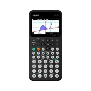
Geometric Probability Distributions on Calculator
A geometric probability distribution is used when you repeatedly perform independent trials until the first success occurs. Each trial has only two possible outcomes—success or failure—and the probability of success remains constant from one trial to the next.
The TI-84 calculator can quickly calculate probabilities for geometric distributions using the geometpdf( and geometcdf( functions.
What Is a Geometric Distribution?
A geometric distribution describes the number of trials needed to obtain the first success in a sequence of independent Bernoulli trials.
For example, suppose a basketball player has a 20% probability of making a free throw on each attempt. If we continue taking free throws until the first successful shot, the number of attempts required follows a geometric distribution.
The probability that the first success occurs on trial x is: P(X=x)=(1−p)x−1p
where:
- X = trial on which the first success occurs
- p = probability of success on each trial
- 1−p = probability of failure
- x = number of trials through the first success
The exponent is x−1 because the first x−1 trials must be failures, followed by a success on trial x.
Example
If: p=0.20
and we want the probability that the first success occurs on the third trial: P(X=3)=(1−0.20)3−1(0.20) =(0.80)2(0.20) =0.128
Therefore, the probability is 0.128, or 12.8%.
Geometric Probability Functions on the TI-84
The TI-84 provides two useful functions:
geometpdf(
The probability mass function (PMF) calculates the probability that the first success occurs on exactly a particular trial.
geometpdf(p,x)
geometcdf(
The cumulative distribution function (CDF) calculates the probability that the first success occurs on or before a particular trial.
geometcdf(p,x)
This distinction is important:
geometpdf→ exactly trial xgeometcdf→ within the first x trials
How to Access Geometric Distribution Functions on a TI-84
To access these functions:
- Turn on the TI-84 calculator.
- Press 2nd.
- Press VARS to open the DISTR menu.
- Scroll through the available distributions.
- Select
geometpdf(orgeometcdf(.
You can then enter the probability of success and the number of trials.
How to Calculate a Geometric PMF on a TI-84
Suppose the probability of success on each trial is: p=0.20
and you want to find the probability that the first success occurs on the third trial.
Step 1: Select geometpdf(
From the distribution menu, select:
geometpdf(
Step 2: Enter the Probability and Trial Number
Enter:
geometpdf(0.2,3)
Then press ENTER.
The calculator returns: 0.128
Therefore: P(X=3)=0.128
or 12.8%.
This means there is a 12.8% probability that the first success will occur exactly on the third trial.
How to Calculate a Geometric CDF on a TI-84
Now suppose you want to determine the probability that the first success occurs within the first four trials.
Using: p=0.20
and: x=4
select geometcdf( and enter:
geometcdf(0.2,4)
The result is: 0.5904
Therefore: P(X≤4)=0.5904
or 59.04%.
In other words, there is approximately a 59.04% probability that the first success occurs during the first four trials.
Understanding the Difference Between PMF and CDF
Consider a geometric distribution with p=0.20.
| Question | TI-84 Function | Interpretation |
|---|---|---|
| First success occurs on trial 3 | geometpdf(0.2,3) | Exactly trial 3 |
| First success occurs by trial 3 | geometcdf(0.2,3) | Trial 1, 2, or 3 |
| First success occurs on trial 5 | geometpdf(0.2,5) | Exactly trial 5 |
| First success occurs by trial 5 | geometcdf(0.2,5) | Any trial from 1 through 5 |
This is one of the most important concepts to understand when using geometric distributions.
Example: First Success on the 5th Trial
Suppose a machine successfully produces a desired product with probability 0.30 on each production attempt.
What is the probability that the first successful product occurs on the fifth attempt?
Here: p=0.30
and: x=5
On the TI-84, enter:
geometpdf(0.3,5)
Using the geometric PMF: P(X=5)=(1−0.30)4(0.30) =(0.70)4(0.30) =0.07203
Therefore, the probability is approximately: 7.20%
Example: First Success Within 5 Trials
Using the same probability: p=0.30
suppose we want the probability that the first success occurs within the first five attempts.
On the TI-84, enter:
geometcdf(0.3,5)
The result is: 0.83193
Therefore: 83.19%
There is approximately an 83.19% probability that at least one success occurs within the first five trials.
Finding the Probability of No Success Within a Given Number of Trials
A useful property of the geometric distribution is: P(X>x)=(1−p)x
For example, suppose: p=0.20
What is the probability that the first success does not occur during the first four trials?
Using the formula: P(X>4)=(1−0.20)4 =0.84 =0.4096
So the probability is 40.96%.
You can also obtain this using the complement of the CDF: P(X>4)=1−P(X≤4)
Since: P(X≤4)=0.5904
we get: 1−0.5904=0.4096
Common Geometric Distribution Questions
When solving geometric probability problems, watch for words that indicate whether you need a PMF or CDF.
“Exactly”
If the question asks:
What is the probability that the first success occurs on the 6th trial?
Use:
geometpdf(p,6)
“Within”
If the question asks:
What is the probability that the first success occurs within 6 trials?
Use:
geometcdf(p,6)
“At most”
If the question asks:
What is the probability that the first success occurs in at most 6 trials?
Use:
geometcdf(p,6)
“More than”
If the question asks:
What is the probability that more than 6 trials are needed?
You can use: P(X>6)=1−P(X≤6)
or calculate:
1-geometcdf(p,6)
Conditions for a Geometric Distribution
A situation can be modeled using a geometric distribution when the following conditions are satisfied:
- There are repeated trials.
- Each trial has two possible outcomes: success or failure.
- The trials are independent.
- The probability of success remains constant.
- The random variable represents the number of trials until the first success.
For example, repeatedly rolling a die until you obtain a 6 can be modeled using a geometric distribution.
The probability of success is: p=61
The probability of failure is: 1−p=65
Mean and Standard Deviation of a Geometric Distribution
The geometric distribution also has useful theoretical properties.
The expected number of trials until the first success is: E(X)=p1
The variance is: Var(X)=p21−p
and the standard deviation is: σX=p1−p
For example, if: p=0.20
then the expected number of trials is: E(X)=0.201=5
So, on average, we would expect the first success to occur after 5 trials.
Geometric Distribution vs. Binomial Distribution
Geometric and binomial distributions both involve repeated Bernoulli trials, but they answer different questions.
| Distribution | Main Question |
|---|---|
| Geometric | How many trials until the first success? |
| Binomial | How many successes occur in a fixed number of trials? |
For example:
Geometric:
“What is the probability that the first success occurs on the 5th attempt?”
Binomial:
“What is the probability of getting exactly 3 successes in 10 attempts?”
Knowing whether the number of trials is fixed or continues until the first success helps determine which distribution to use.
Conclusion
The geometric probability distribution is useful for analyzing the number of trials required to obtain the first success in a sequence of independent trials.
On a TI-84 calculator:
geometpdf(p,x)
calculates the probability that the first success occurs exactly on trial x, while:
geometcdf(p,x)
calculates the probability that the first success occurs on or before trial x.
For example:
geometpdf(0.2,3)
gives the probability of the first success occurring exactly on trial 3, while:
geometcdf(0.2,4)
gives the probability of the first success occurring within the first 4 trials.
Understanding the difference between these two functions will allow you to solve a wide range of geometric probability problems quickly and accurately with a TI-84 calculator.