How to Measure Contingency-Coefficient, when the hypothesis of independence of attributes in a contingency table is rejected by performing a chi-square test, ensures the association between two attributes.

Such kinds of situations are interested to calculate the strength of association and it is a desideratum.  For this, a measure is known as the coefficient of contingency.

The measure of contingency was developed by Karl Pearson in 1904.

The coefficient of contingency is denoted as C.

C=sqrt(χ2/n+ χ2)

Where n is the sample size. The value of C lies between 0 and 1 and never attains 1.

When C=0 indicates complete dissociation. A value near 1 indicates a high degree of association.

In most cases, C calculated when the null hypothesis rejected.

Chi square distribution examples

Introduction to Chi-Square Test

The Chi-Square test in R is a statistical method used to determine if two categorical variables have a significant correlation between them.

The two variables are selected from the same population and labeled as categorically.

Syntax: chisq.test() is a function used to perform the test in R

We reject the null hypothesis if the p-value that comes out in the result is less than a significance level, which is 0.05 usually.

H0: The two variables are independent.

H1: The two variables relate to each other.

Getting Data

data("mtcars")
table(mtcars$carb, mtcars$cyl)

Contigency table from mtcars

    4 6 8
  1 5 2 0
  2 6 0 4
  3 0 0 3
  4 0 4 6
  6 0 1 0
  8 0 0 1

Visulization

library(gplots)
dt<-table(mtcars$carb, mtcars$cyl)
balloonplot(t(dt), main ="Balloon Plot", xlab ="", ylab="",
            label = FALSE, show.margins = FALSE)

Let’s calculate the chi-square value based on chisq.test function

chisq.test(mtcars$carb, mtcars$cyl)

Pearson’s Chi-squared test

data:  mtcars$carb and mtcars$cyl
X-squared = 24.389, df = 10, p-value = 0.006632
Warning message:
In chisq.test(mtcars$carb, mtcars$cyl) :
  Chi-squared approximation may be incorrect

Now you can see the warning because some of the cell frequencies are less than 5.

According Chi-Square test significant difference was observed between tested attributes. However, will check fisher’s exact results also.

Cluster Analysis in R

Fisher’s Exact Test for Count Data

fisher.test(mtcars$carb, mtcars$cyl)
data:  mtcars$carb and mtcars$cyl
p-value = 0.0003345
alternative hypothesis: two.sided

There is no changes in the inferences significant difference was observed between variables, now will check the association of variables.

Let’s visualize Pearson residuals using the package corrplot:

library(corrplot)
chisq<-chisq.test(mtcars$carb, mtcars$cyl)
corrplot(chisq$residuals, is.cor = FALSE)

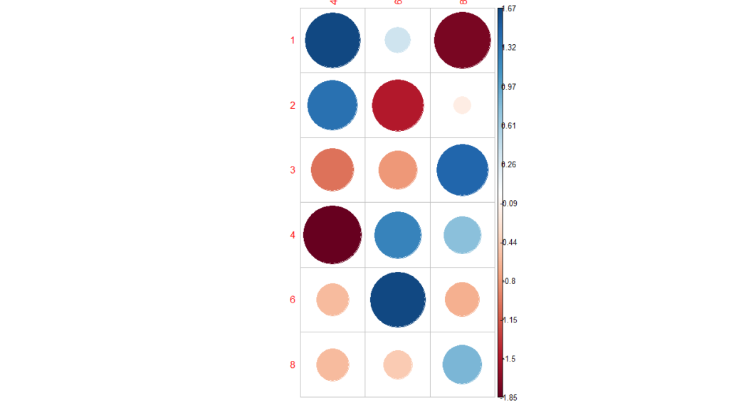
For a given cell, the size of the circle is proportional to the amount of the cell contribution.

The sign of the standardized residuals is also very important to interpret the association between rows and columns.

Positive residuals are in blue and Negative residuals are in red. Based on the above plot, association observed as high.

Customer Segmentation K Means Cluster

Contingency Coefficient

Assocs function fron DescTools returns different association measures simultaneously.

library(DescTools)
Assocs(dt)

estimate  lwr.ci  upr.ci
Phi Coeff.               0.8730       -       -
Contingency Coeff.       0.6577       -       -
Cramer V                 0.6173  0.1778  0.7592
Goodman Kruskal Gamma    0.6089  0.3745  0.8432
Kendall Tau-b            0.4654  0.2846  0.6463
Stuart Tau-c             0.4834  0.2981  0.6687
Somers D C|R             0.4319  0.2650  0.5989
Somers D R|C             0.5015  0.2935  0.7095
Pearson Correlation      0.5746  0.2825  0.7692
Spearman Correlation     0.5801  0.2900  0.7725
Lambda C|R               0.4444  0.1198  0.7691
Lambda R|C               0.2727  0.0000  0.5570
Lambda sym               0.3500  0.1128  0.5872
Uncertainty Coeff. C|R   0.4782  0.3693  0.5870
Uncertainty Coeff. R|C   0.3387  0.2752  0.4022
Uncertainty Coeff. sym   0.3965  0.3220  0.4710
Mutual Information       0.7353       -       -

From the above table Contingency Coefficient value observed as 0.6577, indicates a high association between the tested variables.

Summary

Based on the above analysis, a significant difference was observed between the variables (ie variables are related) and strength of association between the variable is high.

Principal Component Analysis in R