Sentiment analysis in R
Sentiment analysis in R, In this article, we will discuss sentiment analysis using R. We will make use of the syuzhet text package to analyze the data and get scores for the corresponding words that are present in the dataset.
The ultimate aim is to build a sentiment analysis model and identify the words whether they are positive, negative, and also the magnitude of it.
In this article codes are mainly divided into loading data, build a corpus, cleansing text, create term-document matrix, visualization, and sentiment analysis.
Sentiment analysis in R
The following main packages are used in this article
- tm for text mining operations like removing numbers, special characters, punctuations and stop words (Stop words in any language are the most commonly occurring words that have very little value for NLP and should be filtered out
- word cloud for generating the word cloud plot.
- syuzhet for sentiment scores and emotion classification
- ggplot2 for plotting graphs
What is Sentiment Analysis?
Sentiment Analysis is a process of extracting opinions that have different scores like positive, negative or neutral.
Based on sentiment analysis, you can find out the nature of opinion or sentences in text.
Sentiment Analysis is a type of classification where the data is classified into different classes like positive or negative or happy, sad, angry, etc.
Getting data
apple <- read.csv("D:/RStudio/SentimentAnalysis/Data1.csv", header = T)
str(apple)
This dataset contains 1000 observations and 16 variables but we are interested only in one column that is ‘text’.
data.frame': 1000 obs. of  16 variables:
 $ text         : chr  "RT @option_snipper: $AAPL beat on both eps and revenues. SEES 4Q REV. $49B-$52B, EST. $49.1B https://t.co/hfHXqj0IOB" "RT @option_snipper: $AAPL beat on both eps and revenues. SEES 4Q REV. $49B-$52B, EST. $49.1B https://t.co/hfHXqj0IOB" "Let's see this break all timers. $AAPL 156.89" "RT @SylvaCap: Things might get ugly for $aapl with the iphone delay. With $aapl down that means almost all of t"| __truncated__ ... $ favorited    : logi  FALSE FALSE FALSE FALSE FALSE FALSE ... $ favoriteCount: int  0 0 0 0 0 0 0 0 0 0 ...
 $ replyToSN    : chr  NA NA NA NA ... $ created      : chr  "2017-08-01 20:31:56" "2017-08-01 20:31:55" "2017-08-01 20:31:55" "2017-08-01 20:31:55" ...
 $ truncated    : logi  FALSE FALSE FALSE FALSE FALSE FALSE ...
 $ replyToSID   : num  NA NA NA NA NA NA NA NA NA NA ...
 $ id           : num  8.92e+17 8.92e+17 8.92e+17 8.92e+17 8.92e+17 ...
 $ replyToUID   : num  NA NA NA NA NA NA NA NA NA NA ..
Build corpus
Once we loaded the dataset in R, the next step is to load that Vector or text data as a Corpus. We can execute the same based on tm package in R.
library(tm)
corpus <- iconv(apple$text)
corpus <- Corpus(VectorSource(corpus))
inspect(corpus[1:5])
Metadata: corpus specific: 1, document level (indexed): 0
Content: documents: 5
[1] RT @option_snipper: $AAPL beat on both eps and revenues. SEES 4Q REV. $49B-$52B, EST. $49.1B https://t.co/hfHXqj0IOB
[2] RT @option_snipper: $AAPL beat on both eps and revenues. SEES 4Q REV. $49B-$52B, EST. $49.1B https://t.co/hfHXqj0IOB
[3] Let's see this break all timers. $AAPL 156.89
[4] RT @SylvaCap: Things might get ugly for $aapl with the iphone delay. With $aapl down that means almost all of the FANG stocks were down pos…
[5] $AAPL - wow! This was supposed to be a throw-away quarter and AAPL beats by over 500 million in revenue! Trillion dollar company by 2018!
Clean text
In the cleaning process first, we need to convert all the text into lower case. Based on tm_map function can convert text into lower case.
corpus <- tm_map(corpus, tolower)
inspect(corpus[1:5])
Metadata: corpus specific: 1, document level (indexed): 0
Content: documents: 5
[1] rt @option_snipper: $aapl beat on both eps and revenues. sees 4q rev. $49b-$52b, est. $49.1b https://t.co/hfhxqj0iob
[2] rt @option_snipper: $aapl beat on both eps and revenues. sees 4q rev. $49b-$52b, est. $49.1b https://t.co/hfhxqj0iob
[3] let's see this break all timers. $aapl 156.89
[4] rt @sylvacap: things might get ugly for $aapl with the iphone delay. with $aapl down that means almost all of the fang stocks were down pos…
[5] $aapl - wow! this was supposed to be a throw-away quarter and aapl beats by over 500 million in revenue! trillion dollar company by 2018!
Cleaning the text data one of the major parts is removing special characters from the text. This is done using the tm_map() function to replace all kinds of special characters.
corpus <- tm_map(corpus, removePunctuation)
inspect(corpus[1:5])
Metadata: corpus specific: 1, document level (indexed): 0
Content: documents: 5
[1] rt optionsnipper aapl beat on both eps and revenues sees 4q rev 49b52b est 491b httpstcohfhxqj0iob
[2] rt optionsnipper aapl beat on both eps and revenues sees 4q rev 49b52b est 491b httpstcohfhxqj0iob
[3] lets see this break all timers aapl 15689
[4] rt sylvacap things might get ugly for aapl with the iphone delay with aapl down that means almost all of the fang stocks were down pos…
[5] aapl wow this was supposed to be a throwaway quarter and aapl beats by over 500 million in revenue trillion dollar company by 2018
In the text data numbers are commonly occur, we need to remove numbers from the text data.
corpus <- tm_map(corpus, removeNumbers)
inspect(corpus[1:5])
Metadata: corpus specific: 1, document level (indexed): 0
Content: documents: 5
[1] rt optionsnipper aapl beat on both eps and revenues sees q rev bb est b httpstcohfhxqjiob
[2] rt optionsnipper aapl beat on both eps and revenues sees q rev bb est b httpstcohfhxqjiob
[3] lets see this break all timers aapl
[4] rt sylvacap things might get ugly for aapl with the iphone delay with aapl down that means almost all of the fang stocks were down pos…
[5] aapl wow this was supposed to be a throwaway quarter and aapl beats by over million in revenue trillion dollar company by
Stop words are the most commonly occurring words in a language and have very little value in terms of extracting useful information from the text. Need to remove all stopwords from the text before the analysis.
Stop words mean like “the, is, at, on”. stopwords in the tm_map() function supports several languages like English, French, German, Italian, and Spanish.
cleanset <- tm_map(corpus, removeWords, stopwords('english'))
inspect(cleanset[1:5])
Metadata: corpus specific: 1, document level (indexed): 0
Content: documents: 5
[1] rt optionsnipper aapl beat eps revenues sees q rev bb est b httpstcohfhxqjiob
[2] rt optionsnipper aapl beat eps revenues sees q rev bb est b httpstcohfhxqjiob
[3] lets see break timers aapl
[4] rt sylvacap things might get ugly aapl iphone delay aapl means almost fang stocks pos…
[5] aapl wow supposed throwaway quarter aapl beats million revenue trillion dollar company
Depends on your dataset if links contain the dataset remove the same.
removeURL <- function(x) gsub('http[[:alnum:]]*', '', x)
cleanset <- tm_map(cleanset, content_transformer(removeURL))
inspect(cleanset[1:5])
Metadata: corpus specific: 1, document level (indexed): 0
Content: documents: 5
[1] rt optionsnipper aapl beat eps revenues sees q rev bb est b
[2] rt optionsnipper aapl beat eps revenues sees q rev bb est b
[3] lets see break timers aapl
[4] rt sylvacap things might get ugly aapl iphone delay aapl means almost fang stocks pos…
[5] aapl wow supposed throwaway quarter aapl beats million revenue trillion dollar company
Text stemming – which reduces words to their root form
cleanset <- tm_map(cleanset, removeWords, c('aapl', 'apple'))
cleanset <- tm_map(cleanset, gsub,
                   pattern = 'stocks',
                   replacement = 'stock')
cleanset <- tm_map(cleanset, stemDocument)
cleanset <- tm_map(cleanset, stripWhitespace)
inspect(cleanset[1:5])
Metadata: corpus specific: 1, document level (indexed): 0
Content: documents: 5
[1] rt optionsnipp beat ep revenu see q rev bb est b
[2] rt optionsnipp beat ep revenu see q rev bb est b
[3] let see break timer
[4] rt sylvacap thing might get ugli iphon delay mean almost fang stock pos…
[5] wow suppos throwaway quarter beat million revenu trillion dollar compani
Term document matrix
After cleansing the textual content data, the following step is to matter the incidence of every word, to perceive famous or trending topics.
Using the function TermDocumentMatrix() from the textual content mining package, you may construct a Document Matrix – a table containing the frequency of words.
tdm <- TermDocumentMatrix(cleanset)
tdm <- as.matrix(tdm)
tdm[1:10, 1:20]
Docs
 Terms         1 2 3 4 5 6 7 8 9 10 11 12 13 14 15 16 17 18 19 20
   beat        1 1 0 0 1 0 0 0 0  0  0  0  0  0  0  0  0  0  1  0
   est         1 1 0 0 0 2 2 0 0  0  0  0  0  2  0  0  2  2  0  0
   optionsnipp 1 1 0 0 0 0 0 0 0  0  0  0  0  0  0  0  0  0  0  0
   rev         1 1 0 0 0 1 1 0 0  1  0  0  1  0  0  0  1  1  0  0
   revenu      1 1 0 0 1 0 0 0 1  0  0  0  0  0  0  0  0  0  0  0
   see         1 1 1 0 0 0 0 0 0  0  0  0  0  0  0  0  0  0  0  0
   break       0 0 1 0 0 0 0 1 1  1  1  0  0  0  0  0  0  0  0  0
   let         0 0 1 0 0 0 0 0 0  0  0  0  0  0  0  0  0  0  0  0
   timer       0 0 1 0 0 0 0 0 0  0  0  0  0  0  0  0  0  0  0  0
   almost      0 0 0 1 0 0 0 0 0  0  0  0  0  0  1  0  0  0  0  0
Bar plot
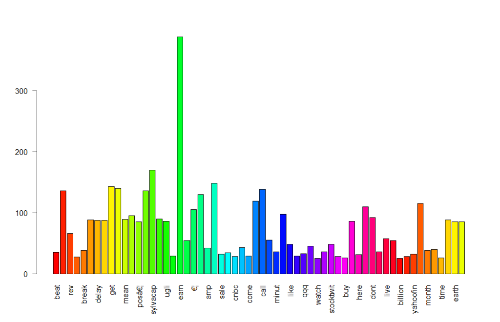
Plotting the words using a bar chart is a good basic way to visualize this word’s frequent data. Simply you can create a bar chart for visualization.
w <- rowSums(tdm)
w <- subset(w, w>=25)
barplot(w,
        las = 2,
        col = rainbow(50))
Word cloud
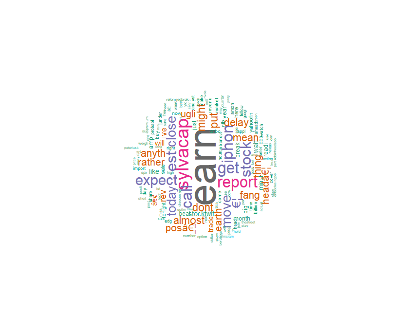
A word cloud is one of the most popular ways to visualize and analyze text data. It’s an image composed of keywords found within a body of text, where the size of each word indicates its count in that body of text.
Latest data science job vacancies
Use the word frequency data frame (table) created previously to generate the word cloud.
library(wordcloud)
w <- sort(rowSums(tdm), decreasing = TRUE)
set.seed(222)
wordcloud(words = names(w),
          freq = w,
          max.words = 150,
          random.order = F,
          min.freq = 5,
          colors = brewer.pal(8, 'Dark2'),
          scale = c(5, 0.3),
          rot.per = 0.7)
library(wordcloud2)
w <- data.frame(names(w), w)
colnames(w) <- c('word', 'freq')
wordcloud2(w,
           size = 0.7,
           shape = 'triangle',
           rotateRatio = 0.5,
           minSize = 1)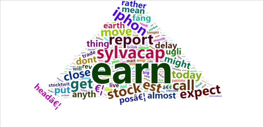
Sentiment analysis
We discussed earlier sentiments can be classified as positive, neutral, or negative. They can also be represented on a numeric scale, to better express the degree of positive or negative strength of the sentiment contained in a body of text.
This example uses the Syuzhet package for generating sentiment scores, which has four sentiment dictionaries and offers a method for accessing the sentiment extraction tool developed in the NLP group at Stanford.
The get_sentiment function accepts two arguments: a character vector (of sentences or words) and a method. The selected method determines which of the four available sentiment extraction methods will be used. The four methods are syuzhet (this is the default), bing, afinn and nrc.
Each method uses a different scale and hence returns slightly different results.
library(syuzhet)
library(lubridate)
library(ggplot2)
library(scales)
library(reshape2)
library(dplyr)
Getting Data
apple <- read.csv("D:/RStudio/SentimentAnalysis/Data1.csv", header = T)
tweets <- iconv(apple$text)
Obtain sentiment scores
s <- get_nrc_sentiment(tweets)
head(s)
anger anticipation disgust fear joy sadness surprise trust negative positive
1     0            0       0    0   0       0        0     0        0        1
2     0            0       0    0   0       0        0     0        0        1
3     0            0       0    0   0       0        1     0        0        0
4     1            0       2    2   0       1        0     0        3        0
5     0            0       0    0   0       0        0     0        0        0
6     0            0       0    0   0       0        0     0        0        0
Its ranging from anger to trust, Negative and Positive.
get_nrc_sentiment(ugly)
anger anticipation disgust fear joy sadness surprise trust negative positive
 0            0       1    0   0       0        0     0        1        0
Ugly has scores on disgust and negative.
Bar plot
barplot(colSums(s),
        las = 2,
        col = rainbow(10),
        ylab = 'Count',
        main = 'Sentiment Scores Tweets')
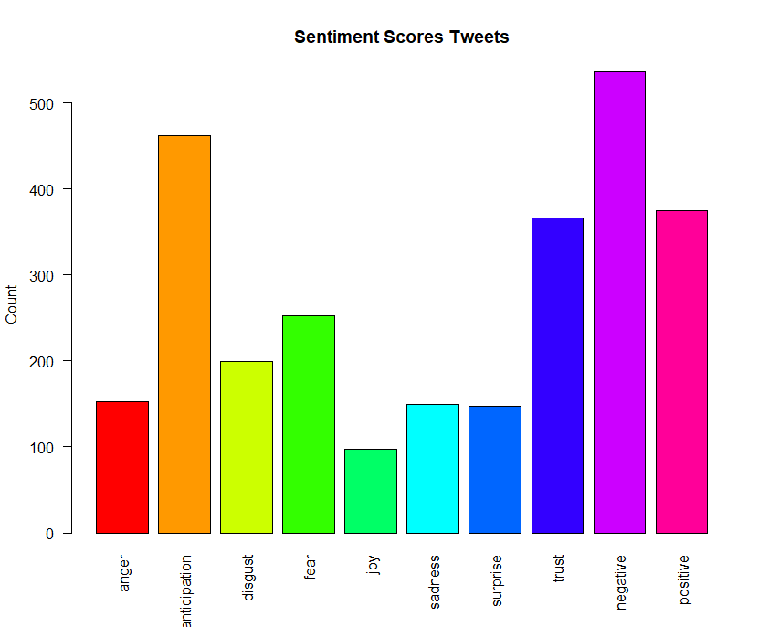
Sentiment scores more on negative followed by anticipation and positive, trust and fear.
Conclusion
This article explained reading text data into R, corpus creation, data cleaning, transformations and explained how to create a word frequency and word clouds to identify the occurrence of the text.
Identification of sentiment scores, which proved useful in assigning a numeric value to strength (of positivity or negativity) of sentiments in the text and allowed interpreting score of the text.
