How to perform ANCOVA in R
ANCOVA in R, Analysis of covariance is used to measure the main effect and interaction effects of categorical variables on a continuous dependent variable while controlling the effects of selected other continuous variables which is co-vary with the dependent.
ANCOVA in R
We can take one of the simple examples to conduct ANCOVA in R. Identify the studying technique has an impact on exam scores by using the following parameters.
Technique: Interested variable to analyze (independent variable) the effect of techniques affect the score or not.
Grade: The covariate that we want to take into account, current grade of the student.
Score: The response variable (dependent variable) interested in analyzing
Let’s create a data frame contains the information for 90 students that were randomly split into three groups of 30.
Here we mentioned three techniques that are coded as A, B, and C.
Let’s make use of set.seed for repeatability.
LSTM Network in R » Recurrent Neural network »
set.seed(123)
Create the data set in R
  technique    grade     exam
1         A 73.47893 85.08908
2         A 83.09936 85.09367
3         A 74.84477 76.24713
4         A 82.08737 70.51951
5         A 73.10378 79.11569
6         A 68.68576 73.62893
Explore the Data
Once we have the dataset for analysis, we need to examine the data set first, like extreme values NA values etc.
Let’s create a summary of the current dataset.
summary(data)
technique             grade            exam
 Length:90          Min.   :65.02   Min.   :60.79
 Class :character   1st Qu.:69.43   1st Qu.:75.46
 Mode  :character   Median :74.21   Median :83.06
                    Mean   :74.55   Mean   :82.03
                    3rd Qu.:79.65   3rd Qu.:88.60
                    Max.   :84.67   Max.   :94.91
Here we can see the minimum, maximum, mean and average values. No need to make any extra changes here because our dataset as good it is.
The standard deviation is one of the important factors, we need to get the dispersion of the current dataset.
Linear optimization using R » Optimal Solution »
library(dplyr)
   data %>%
            group_by(technique) %>%
            summarise(mean_grade = mean(grade),
            sd_grade = sd(grade),
            mean_exam = mean(exam),
            sd_exam = sd(exam))
technique mean_grade sd_grade mean_exam sd_exam 1 A 74.08737 5.829004 82.72918 8.682884 2 B 74.71526 5.274380 77.47258 9.658907 3 C 74.84389 6.580034 85.89504 3.567625
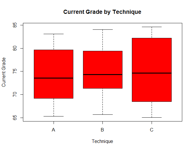
We can see that the mean and the standard deviations of the current grade is more or less the same.
We can make use of boxplots for the visualization
boxplot(exam ~ technique,
data = data,
main = "Score by Technique",
xlab = "Technique",ylab = "Score",
col = "red",border = "black")

Similarly, we can also use boxplots to visualize the distribution of current grades.
boxplot(grade ~ technique,data = data,
main = "Current Grade by Technique",
xlab = "Technique",ylab = "Current Grade",
col = "red",border = "black")

Model Assumptions
When we do ANCOVA, we need to check some basic assumptions.
1. The covariate and the treatment are independent
Need to verify that the covariate in this case grade and the technique are independent to each other.
2.Homogeneity of variance
Verify the variances among the groups is equal or not
For assumption 1 we can make use of the ANOVA model.
Exploratory Data Analysis (EDA) » Overview »
Let’s fit the model,
model <- aov(grade ~ technique, data = data)
summary(model)
Df Sum Sq Mean Sq F value Pr(>F)
technique    2    9.8    4.92    0.14  0.869
Residuals   87 3047.7   35.03
The p-value is 0.869 that is greater than 0.05, so the covariate grade and the treatment technique are independent to each other.
For assumption 2, we can make use of Levene’s Test,
library(car)
leveneTest(exam~technique, data = data)
      Df F value    Pr(>F)
group  2  13.752 6.464e-06 ***
      87
---
Signif. codes:  0 ‘***’ 0.001 ‘**’ 0.01 ‘*’ 0.05 ‘.’ 0.1 ‘ ’ 1
The p-value of the test is 6.464e-06, which indicates that the variances among the groups are not equal. It indicates the need to transform the exam variable for the equal group variance.
However, for illustration purposes, we are continuing with the existing dataset and are not much interested in unequal variances.
Principal component analysis (PCA) in R »
Fit analysis of covariance model ANCOVA in R
library(car)
ancova_model <- aov(exam ~ technique + grade, data = data)
Anova(ancova_model, type="III")
Anova Table (Type III tests)
Response: exam
            Sum Sq Df F value    Pr(>F)
(Intercept) 3492.4  1 57.1325 4.096e-11 ***
technique   1085.8  2  8.8814 0.0003116 ***
grade          4.0  1  0.0657 0.7982685
Residuals   5257.0 86
---
Signif. codes:  0 ‘***’ 0.001 ‘**’ 0.01 ‘*’ 0.05 ‘.’ 0.1 ‘ ’ 1
From this result, we can easily conclude that while controlling grade variable still technique variable is statistically significant. It indicates that the technique variable has significantly contributed to the model.
Now we want to know which techniques are different from each other.
Make usage multi-comp package for pairwise comparison.
Cluster Meaning-Cluster or area sampling in a nutshell »
library(multcomp)
ancova_model <- aov(exam ~ technique + grade, data = data)
postHocs <- glht(ancova_model, linfct = mcp(technique = "Tukey"))
summary(postHocs)
Simultaneous Tests for General Linear Hypotheses
Multiple Comparisons of Means: Tukey Contrasts
Fit: aov(formula = exam ~ technique + grade, data = data)
Linear Hypotheses:
           Estimate Std. Error t value Pr(>|t|)
B - A == 0   -5.279      2.021  -2.613   0.0284 *
C - A == 0    3.138      2.022   1.552   0.2719
C - B == 0    8.418      2.019   4.170   <0.001 ***
---
Signif. codes:  0 ‘***’ 0.001 ‘**’ 0.01 ‘*’ 0.05 ‘.’ 0.1 ‘ ’ 1
(Adjusted p values reported -- single-step method)
Now it’s clear a significant difference was observed between the pairs B vs A and C vs B.
Conclusion
From the above Technique-A and Technique-C are significantly better than B.


