Naive Bayes Classifier in Machine Learning
Naive Bayes Classifier in Machine Learning, we are going to discuss the prediction model based on Naive Bayes classification. The prediction model based on the Naive Bayes classification will be discussed in this lesson.
Naive Bayes is a classification method based on Bayes’ Theorem and the assumption of predictor independence.
The Naive Bayes model is simple to construct and is especially good for huge data sets. Consider Naive classification if you have a large dataset.
Naive Bayes Classifier in Machine Learning Process Flow
Take an example, Imagine because of current weather, cricket match will happen or not? Now, we need to classify whether players will play the match or not based on weather conditions.
Convert the data set into a frequency table
1) Create a Likelihood table by finding the probabilities like play the match or not
2) Based on the Naive Bayes equation calculate the posterior probability for each class. The highest posterior probability in each class is the outcome of the prediction.
3) It is easy to use and fast to predict the class of test data set.
It performs well in the case of categorical input variables compared to the numerical variable(s).
Its required independent predictor variables for better performance.
Let’s see, how to execute Naïve Bayes classification in R?
Load libraries
library(naivebayes)
library(dplyr)
library(ggplot2)
library(psych)
Getting Data
data <- read.csv("D:/RStudio/NaiveClassifiaction/binary.csv", header = T)
head(data)
Launch Thickness Appearance Spreading Rank 0 6 9 8 2 0 5 8 7 2 0 8 7 7 2 0 8 8 9 1 0 9 8 7 2 0 7 7 7 2
Let us understand the dataset, the dataset contains 5 columns.
Launch- Response variable, 0 indicates product not launched and 1 indicates the product is launched
Thickness-product thickness score
Appearance-product appearance score
Spreading- product spreading score
Rank-Rank of the product
Frequency Identification
Let’s calculate the frequency of the response variable under each rank. The minimum frequency of each class is 5 required for analysis.
xtabs(~Launch+Rank, data = data)
Rank
    Rank
Launch  1  2  3
     0 12 21 13
     1 21 15 13
In this all-cell frequencies are greater than 5 and ideal for further analysis.
Now just look at each variable class based on the str function
str(data)
data.frame':  95 obs. of  5 variables:
 $ Launch             : int  0 0 0 0 0 0 0 0 0 0 ...
 $ Thickness          : int  6 5 8 8 9 7 8 8 8 8 ...
 $ ColourAndAppearance: int  9 8 7 8 8 7 9 7 9 9 ...
 $ EaseOfSpreading    : int  8 7 7 9 7 7 8 7 9 8 ...
 $ Rank               : int  2 2 2 1 2 2 2 2 1 2 ...
Now you can see the data frame contains 95 (still small dataset you can try Naive Bayes for large datasets) observations of 5 variables.
The columns Launch and Rank are stored as integer variables. If these two variables appear as integer needs to convert into factor variables.
tidyverse in R complete tutorial
data$Rank <- as.factor(data$Rank)
data$Launch <- as.factor(data$Launch)
One of the assumptions in the nave Bayes classification is that the independent variables are not highly correlated.
Remove the rank column in this scenario and test the predictor variables’ association.
Visualization
pairs.panels(data[-1])

Low correlation was observed between independent variables.
Visualize the data based on ggplot
data %>%
         ggplot(aes(x=Launch, y=Thickness, fill = Launch)) +
         geom_boxplot() +theme_bw()+
         ggtitle("Box Plot")

The product got the highest score in the thickness got launched in the market.
data %>%
ggplot(aes(x=Launch, y=Appearance, fill = Launch)) +
geom_boxplot() +theme_bw()+
ggtitle("Box Plot")
data %>%
  ggplot(aes(x=Launch, y=Spreading, fill = Launch)) +
  geom_boxplot() +theme_bw()+
  ggtitle("Box Plot")

Data Partition
Let’s create train and test data sets for training the model and testing.
set.seed(1234)
ind <- sample(2, nrow(data), replace = T, prob = c(0.8, 0.2))
train <- data[ind == 1,]
test <- data[ind == 2,]
Naive Bayes Classification
Naive Bayes Classification in R
model <- naive_bayes(Launch ~ ., data = train, usekernel = T)
model plot(model)
You can try to use kernel = T without also, based on model accuracy you can adjust the same.

Product received rank 1 score launch chances are very high and products received rank 3 also have some chances to a successful launch.
Prediction
p <- predict(model, train, type = 'prob')
head(cbind(p, train))
        0            1     Launch Thickness Appearance Spreading Rank
1 0.9999637 3.629982e-05      0         1          9         8    2
2 0.9998770 1.229625e-04      0         1          8         7    1
3 0.9998804 1.196174e-04      0         1          7         7    1
4 0.9997236 2.764280e-04      0         1          8         9    1
6 0.9998804 1.196174e-04      0         1          7         7    1
7 0.9999637 3.629982e-05      0         1          9         8    2
Basis first row, Low thickness, high appearance, Spreading, and Rank score 2, has a very low chance of product launch.
Confusion Matrix – train data
p1 <- predict(model, train)
 (tab1 <- table(p1, train$Launch))
p1   0  1
   0 28  2
   1  7 37
1 - sum(diag(tab1)) / sum(tab1)
0.1351351
Misclassification is around 14%.
Training model accuracy is around 86% not bad!.
What is the minimum number of units required in an experimental design
Confusion Matrix – test data
p2 <- predict(model, test)
 (tab2 <- table(p2, test$Launch))
p2   0  1
   0  8  0
   1  3 10
1 - sum(diag(tab2)) / sum(tab2)
0.1428571
Conclusion
Misclassification in test data is roughly 14%, according to Naive Bayes Classification in R.
In the train test, you can improve model accuracy by adding more observations.
Don’t forget to show your love, Please Subscribe the Newsletter and COMMENT below!
[newsletter_form type="minimal"]


Is there a download for the .csv file?
Yes, you can access it from the below link.
https://github.com/finnstats/finnstats
Thanks for response. I can see file for “D:/RStudio/NaiveClassifiaction/binary.csv” but don’t see sample file for “D:/RStudio/NaiveClassifiaction/binary.csv”
Please download the file from the below link and change the working directory location accordingly.
https://github.com/finnstats/finnstats/blob/main/binary.csv
Sorry, one last time. Your RStudio/NaiveClassifiaction/binary.csv blog
uses the file name “binary.csv” The one you pointed to is about college admittance from the Logistic Regression blog (400 records).. The one I am looking for is about launch, thickness, appearance (95 records) in the Naive Classification blog. Thanks
This one:
data.frame’: 95 obs. of 5 variables:
$ Launch : int 0 0 0 0 0 0 0 0 0 0 …
$ Thickness : int 6 5 8 8 9 7 8 8 8 8 …
$ ColourAndAppearance: int 9 8 7 8 8 7 9 7 9 9 …
$ EaseOfSpreading : int 8 7 7 9 7 7 8 7 9 8 …
$ Rank : int 2 2 2 1 2 2 2 2 1 2 …
Ok got it…Please find the link.
https://github.com/finnstats/finnstats/blob/main/binary-Naive.csv
That’s it thanks…
I still don’t quite understand the model, yet. But, shouldn’t these variables be train$Launch vice *$admit?
p1 <- predict(model, train)
(tab1 <- table(p1, train$admit))
p2 <- predict(model, test)
(tab2 <- table(p2, test$admit))
Yes, You are right…Corrected now, Thanks a lot…
Thanks for the blog. I learned a lot from it.
Any advice on how to get rid of this error message in the Data Partition section:
Code:
ind <- sample(2, nrow(data), replace = TRUE, prob = c(0.8, 0.2))
Console Output:
Error in sample.int(x, size, replace, prob) : invalid 'size' argument
Thanks!
Lokks like instead of sample() its loading sample.int().
If you loaded tidyverse package try to remove and call this function again.
Hope this will help you…